

0 引言
钢铁业是国民经济的基础,在工业化进程中起到不可替代的作用[1]。卫星热红外影像可以客观反映地表温度信息,已经广泛应用于城市热岛[2,3]、工业热污染[4]等热效应研究中。近年来,研究者提出运用卫星热红外数据中高温异常像素面积建立生产热辐射模型,来监测钢铁厂月度生产状态[5],初步证实了运用热红外遥感表面温度结果评价钢铁厂产能的可能性,为进一步建立实际产量的估算模型奠定了理论基础。但生产热辐射模型[5]只考虑高温像素面积,未考虑高温像素的分布情况及产生的原因,将所有高温像素纳入生产区面积中,可能对产量评价的结果产生影响。分析可知,钢铁厂区内高温像素分布模式反映生产情况不同。为此,本文提出基于热红外表面温度反演的钢铁企业炼钢月产量估算模型(steelmaking monthly production estimation model,SMPE),该模型结合景观指数[6]理论方法,依据卫星热红外表面温度反演结果和厂区矢量数据,分别得到炼钢生产表面温度异常值和热力景观分布参数,建立钢铁企业炼钢月产量估算模型。为提高精度,对表面温度分级结果中表面孤立温度区开展处理,去除噪声以保证模型的精度。最后,以华中地区某钢铁企业A及华北地区某钢铁企业B为研究对象开展钢铁企业炼钢月产量估算模型的验证。实验结果表明,本文构建的企业A估算模型的决定系数为0.903,后验差检验等级为二级; 企业B估算模型的决定系数为0.905,后验差检验等级为二级,模型拟合效果较好。
炼钢月产量是衡量钢铁企业生产状况的重要指标,对其进行监测和评估可为我国钢铁行业供给侧结构性改革提供发展依据,并对疫情后我国经济有序平稳发展提供有力保障。本文的研究可以辅助监测国内外钢铁企业生产状况,及时、客观形成对国际钢铁行业生产状态的监测和产量的估算,也有望进一步拓宽热红外卫星遥感的应用。
1 研究方法
图1
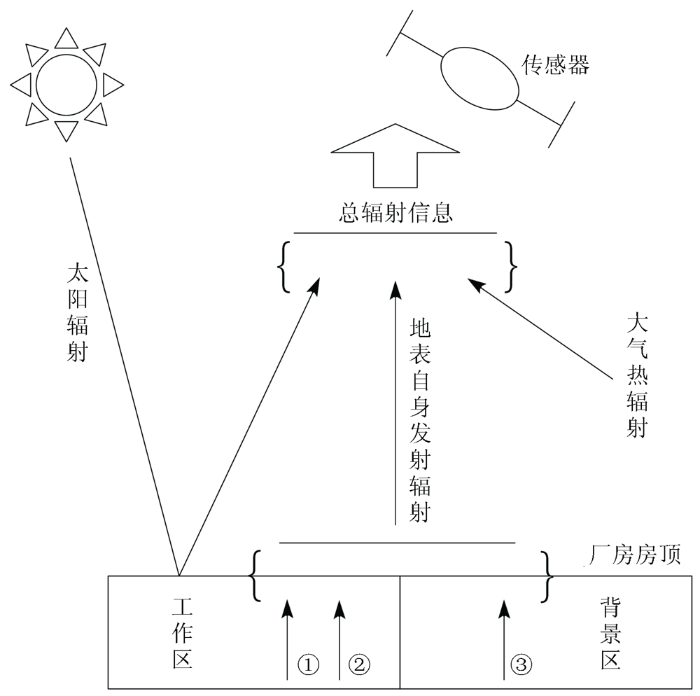
图1
炼钢厂厂房热辐射示意图
Fig.1
Schematic diagram of thermal radiation of steelmaking workshop
1.1 卫星热红外遥感数据
1.2 钢铁企业SMPE模型
采用辐射传输方程法来反演钢铁厂的表面温度后,对结果进行表面温度分级,结合厂房矢量数据获取表面温度异常值与热力景观分布参数,最终建立钢铁企业SMPE模型。试验的具体流程如图2所示。
图2

图2
炼钢月产量估算模型建模流程图
Fig.2
The modeling workflow of steelmaking monthly production estimation model
1.2.1 表面温度分级
以钢铁厂区内表面温度最大值与最小值作为分割区间,依据“均值-标准差”法对研究区进行表面温度分级[23],计算公式为:
式中: T为像元温度,℃; Tmean为研究区表面温度均值,℃; SD为研究区表面温度标准差值,℃。
1.2.2 表面孤立温度区处理
厂区进行表面温度分级后,可能存在由单像素构成的温度分级区,若不加以处理会对最终结果产生不利影响。因此,本文提出运用箱线图(boxplot)方法去除表面孤立温度区中的噪声。
1.2.3 表面温度异常值
剔除噪声后,以表面温度分级结果为基础,对厂房内部进一步分割,厂房内高温区为工作区,厂房内中温区与低温区为背景区,以此为基础来统计表面温度异常值(Tα),计算公式为:
式中: Thigh为工作区表面温度均值,℃; Tback为背景区的表面温度均值,℃。
1.2.4 热力景观分布参数
景观格局指数可定量描述热力景观格局[22],也可以对热力景观格局中温度变化的原因进行表述[25]。斑块是景观格局的基本组成单元,是指不同于周围背景的、相对均质的区域[26]。剔除噪声后,以表面温度分级结果为基础,统计研究区内高温(high temperature,h)、中温(middle temperature,m)、低温(low temperature,l)3类斑块。进一步利用厂房矢量数据将企业内部的高温斑块分为高温工作斑块(high temperature production,hp)和高温非工作斑块(high temperature non-production,hnp)2类(高温非工作斑块主要包括停车场等易产生高温的场所)。通过各参数与实际产量的相关性分析结果来确定热力景观分布参数。表1为钢铁企业各类斑块的数量与月产量实际值的相关性。
表1 参数与月产量实际值相关性
Tab.1
| 参数 | 含义 | 与实际值 间相关性 |
|---|---|---|
| Shp/S | 高温工作斑块面积/总体斑块面积 | 0.817 |
| NPhp | 高温工作斑块数目 | 0.574 |
| NPhnp | 高温非工作斑块数目 | -0.704 |
| NPm | 中温斑块数目 | 0.464 |
| NPl | 低温斑块数目 | -0.339 |
| NP | 总体斑块数目 | -0.087 |
| |NPhp- NPhnp- NPl |/NP | — | -0.920 |
| |NPhp- NPl |/NP | — | -0.841 |
| |NPhp- NPhnp |/NP | — | 0.816 |
| |NPhp- NPhnp- NPm |/NP | — | 0.420 |
| |NPhp- NPm |/NP | — | 0.403 |
炼钢厂中,hp越多,说明处于工作状态的区域越多,但一般来说,hp与其他类型的斑块相比更为集中,钢铁厂区hp数量越多时,hp与hnp,l之间数量的差值越小,说明企业内部生产场所越多,因此月产量值则越高。因此,hp与其他类型斑块差值为负数,|NPhp- NPhnp- NPl |/NP与月产量实际值呈现强的负相关(-0.920)。综合表1的结果,选用Shp/S及|NPhp- NPhnp- NPl |/NP作为热力景观分布参数来参与炼钢月产量估算模型的构建。
1.2.5 模型建立
将表面温度异常值Tα与热力景观分布参数结合,可以反映钢铁企业炼钢的月度生产状态。基于此,建立SMPE估算公式为:
式中: Tα为钢铁企业内的表面温度异常值,℃; β1,β2及bM为需要拟合的参数值,万t。
1.3 精度验证与置信区间
1.3.1 SMPE精度验证
后验差检验是对残差(e)分布的统计特性进行检验,由后验差比值C和小误差概率P共同描述[29]。在研究中,收集钢铁企业实际产量,统计SMPE估算的月产量值,计算公式为:
式中:
指标C值越小表明模型计算的产量值与产量实际值之差的离散程度小。以K倍S1为标准值,统计残差与残差均值之差的绝对值小于标准值的频率,P值越大表明频率越大。C值与P值对应的拟合精度等级见表2。
表2 拟合精度等级
Tab.2
| 精度等级 | C值 | P值 |
|---|---|---|
| 1级(良好) | C<0.35 | P>0.95 |
| 2级(合格) | 0.35≤C<0.50 | 0.80<P≤0.95 |
| 3级(勉强) | 0.50≤C<0.65 | 0.70<P≤0.80 |
| 4级(不合格) | C≥0.65 | P≤0.70 |
1.3.2 SMPE结果置信区间
SMPE结果与实际值存在偏差,置信区间包含计算值的波动范围,可以传递更详细的信息,具有重要意义[30]。假设SMPE值如式(11)所示,则在1-α(α为显著性水平)的置信度下,钢铁企业第i月的产量实际值落在产量估算值的如下置信区间(式(15))内,具体公式为:
式中:
2 钢铁企业结果分析
本文选取华中地区某钢铁企业A及华北地区某钢铁企业B为研究对象。企业A为一所典型大型钢铁企业; 企业B为一所典型的小型钢铁企业。
2.1 企业A研究区结果分析
2.1.1 企业A研究区模型参数获取
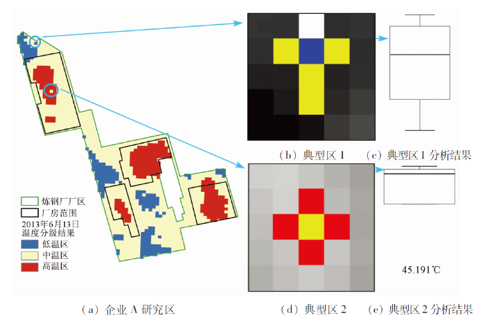
得到企业A表面温度反演结果后,利用公式(1)计算企业A的表面温度分级结果。然后提取表面温度分级后的孤立温度区及其四邻域的温度值,利用箱线图方法来判断表面孤立温度区是否为噪声(表3和图3)。图3(c)为图3(a)中提取的表面温度值的箱线图分析结果,该表面孤立温度区及其四邻域表面温度值均在箱线图的上-下限范围内,因此判断此表面孤立温度区不是噪声,应予以保留; 图3(e)为图3(d)中提取的表面温度值的箱线图分析结果,可以发现表面孤立温度区的温度值为45.191 ℃,低于箱线图的下限值,因此判断此表面孤立温度区为噪声需要予以剔除(表3)。基于剔除噪声后的表面温度分级结果,利用厂房矢量获得工作区与背景区,然后利用式(2)计算得到表面温度异常值Tα。同时,将厂区分为高温工作斑块、高温非工作斑块、中温斑块以及低温斑块这四种类型,统计斑块的数量及面积来计算出热力景观分布参数。
表3 表面孤立温度区及其四邻域表面温度值
Tab.3
| 图 | 表面孤立温度 区温度值/℃ | 四邻域表面温度值/℃ | 结果 | |||
|---|---|---|---|---|---|---|
| 38.764 | 38.982, | 39.175, | 39.120, | 38.614 | 保留 | |
| 45.191 | 47.324, | 47.274, | 47.196, | 46.680 | 剔除 | |
图3
2.1.2 研究区企业A的模型构建及验证
本文利用25个月份的Landsat系列影像数据来进行炼钢月产量估算模型的构建及验证。用前17个月份的数据来拟合模型中的参数,后8个月份的数据来验证模型精度。
利用拟合后的炼钢月产量估算模型计算后8个月的SMPE,然后通过后验差检验方法来说明模型的精度等级。得到残差计算表(表4)及变化曲线图(图4)。计算得出企业A的SMPE精度验证参数见表5。表中,指标C=0.388,<0.5,评定结果为2级(合格); 指标P=1,>0.95,评定结果为1级(良好),说明模型拟合效果好。然后利用式(11)—(15)计算出SMPE的置信区间。显著性水平α取为0.05,样本数n=17,查找t界值表可知
表4 验证用实际值与SMPE值残差及残差百分比
Tab.4
| 时间 | 残差Yj- | 残差百分比(Yj- |
|---|---|---|
| 2017年2月 | -4.409 | -3.50% |
| 2017年10月 | -1.889 | -1.35% |
| 2017年12月 | -0.601 | -0.45% |
| 2018年7月 | -4.372 | -3.13% |
| 2018年9月 | -3.800 | -2.76% |
| 2018年10月 | 1.736 | 1.24% |
| 2018年11月 | 1.554 | 1.12% |
| 2020年2月 | -7.575 | -6.47% |
| 均值 | -2.419 | -1.91% |
图4
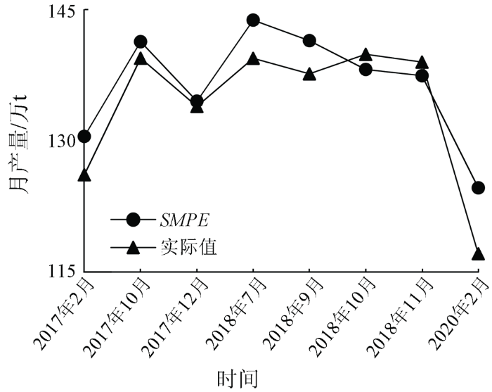
图4
验证用实际值与SMPE值曲线
Fig.4
The curves of actual values for validation and SMPE values
表5 企业A的SMPE精度验证参数
Tab.5
| 参数 | S1 | S2 | C | P | ||
|---|---|---|---|---|---|---|
| 数值 | 134.080 | -2.419 | 7.772 | 3.019 | 0.388 | 1 |
图5
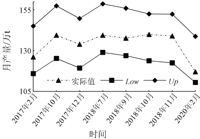
图5
SMPE值置信区间(置信度=95%)
Fig.5
Confidence interval of SMPE (Confidence level = 95%)
2.2 企业B研究区结果分析
2.2.1 企业B研究区模型参数获取
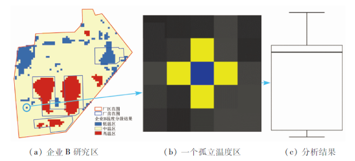
在企业B研究区表面温度反演结果的基础上,利用式(1)对企业B研究区进行温度分级(图6(a)),然后利用箱线图方法来判断表面孤立温度区温度值与其四邻域表面温度值之间的关系。图6(b)为企业B研究区2016年5月表面温度分级结果中的一个孤立温度区,图6(c)为对其温度及其四邻域温度值进行箱线图分析的结果,结果表明,此表面孤立温度区的温度值在箱线图的上下限之间,判断为非噪声,可以保留。排除噪声的干扰后,在表面温度分级结果的基础上,结合企业B研究区厂房矢量数据将厂房划分为工作区与背景区,并利用式(2)计算得到表面温度异常值Tα。同时利用排除孤立噪声后的表面温度分级结果及厂房矢量将企业B研究区划分为高温工作斑块、高温非工作斑块、中温斑块以及低温斑块,统计出上述斑块的数量及面积来计算出热力景观分布参数。
图6
2.2.2 企业B研究区模型构建及分析
利用17个月份的Landsat系列遥感影像数据来构建企业B的月产量估算模型。用前12个月份的数据来拟合模型中的有关参数,后5个月份的数据来验证模型的精度等级,并计算出模型计算值的置信区间。
采用最小二乘法拟合炼钢月产量估算模型中参数值,得: β1= -8.672 万t/℃,β2= 16.916 万t/℃,bM= 86.501 万t。
代入式(3)后得到企业B炼钢月产量估算模型,公式为:
表6 验证用实际值与SMPE残差及残差百分比
Tab.6
| 时间 | 残差Yj- | 残差百分比(Yj- |
|---|---|---|
| 2013年7月 | 3.163 | 4.52% |
| 2013年8月 | 3.369 | 4.22% |
| 2014年7月 | 0.770 | 1.01% |
| 2016年5月 | 1.019 | 1.39% |
| 2017年4月 | -0.826 | -1.06% |
| 均值 | 1.499 | 2.02% |
图7

图7
验证用炼钢月产量实际值与SMPE曲线
Fig.7
The curves of actual values for validation and SMPE values
表7 企业B SMPE模型精度验证参数
Tab.7
| 参数 | S1 | S2 | C | P | ||
|---|---|---|---|---|---|---|
| 均值 | 75.528 | 1.499 | 3.604 | 1.576 | 0.438 | 1 |
然后利用式(11)—(15)计算出SMPE的置信区间。显著性水平α取为0.05,样本数n=12,查找t界值表可知
图8
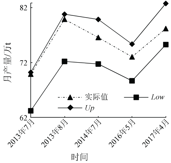
图8
SMPE值置信区间(置信度=95%)
Fig.8
Confidence interval of SMPE (Confidence level = 95%)
3 结论
本文利用卫星热红外遥感数据反演得到厂区热量平衡界面温度后,采用均值-标准差方法对表面温度反演结果进行温度分级,排除噪声干扰后,结合厂房矢量数据对表面温度分级的结果做进一步的分割,从而得到表面温度异常值与热力景观分布参数。然后建立钢铁企业炼钢月产量估算模型(SMPE),结合钢铁企业炼钢月产量实际数据,通过最小二乘算法计算出SMPE模型中的参数值。通过后验差检验的方法来判断模型的拟合精度等级,同时计算出SMPE在95%置信度下的置信区间。通过试验得到以下结论:
1)SMPE与炼钢月产量实际值的变化趋势一致,可以用SMPE来描述钢铁企业的月度生产状态,从整体上反映钢铁企业炼钢月产量的增减情况。
2)从后验差检验法的结果可知,利用有限的钢铁企业实际产量建立的炼钢月产量估算模型具有良好的月产量估算能力,且在95%的置信度下,月产量实际值落在SMPE的置信区间内,说明可以用SMPE来表示月产量实际值,解决实际值缺失的问题,从而实现对钢铁企业的整体生产状态的掌控。
3)本文选取大型钢铁企业A与小型钢铁企业B为研究对象,模型估算的月产量值与月产量实际值之间存在一定的偏差,但从残差百分比的结果来看,偏差在可接受的范围内,说明SMPE适用于不同规模的钢铁企业。
本文结合景观指数建立钢铁企业SMPE模型,通过华中和华北两个钢铁企业的炼钢月产量估算试验说明模型的正确性和适用性,对拓展热红外遥感应用面,及时监测钢铁企业炼钢产量,掌握钢铁企业生产状态具有一定的参考和帮助。但受限于现阶段的实验条件,无法对炼钢厂厂房房顶的真实表面温度开展实地观测,缺少不同风速、不同时间段工作区与背景区厂房顶的实际表面温度差异数据,因此只能在假设工作区与背景区背景热辐射相同的前提下开展实验,在后续的研究中,需要通过实地观测数据来解释工作区与背景区热辐射的真实差异。
参考文献
The Chinese steel industry:Recent developments and prospects
[J].DOI:10.1016/S0301-4207(00)00026-X URL [本文引用: 1]
The impacts of the expansion of urban impervious surfaces on urban heat islands in a coastal city in China
[J].DOI:10.3390/su12020475 URL [本文引用: 1]
基于多源遥感数据的城市环境宜居性研究——以北京市为例
[J].
A study of the livability of urban environment based on multi-source remote sensing data:A case study of Beijing City
[J].
Assessment of hotspots using sparse autoencoder in industrial zones
[J].
DOI:10.1007/s10661-019-7572-3
PMID:31222399
[本文引用: 1]

Remote sensing satellite systems can be used to detect industrial zones by means of thermal infrared bands. There are several satellite systems loaded with thermal infrared sensors such as Landsat and Advanced Spaceborne Thermal Emission and Reflection Radiometer (ASTER). In this study, ASTER thermal infrared data were converted to land surface temperature (LST) in order to determine hotspots caused by industrial zones. High LST values surrounded by low LST values are called hotspots here. These hotspots can be determined by applying different methodologies. One of these methods of sparse autoencoder can be used to indicate hotspots using different sizes of hidden layers. The principle of sparse autoencoder depends on unlabeled data in unsupervised learning. It does not need any information about labeled data as in supervised learning. The autoencoder reproduces its output with the same dimensions as the input image by managing the size of the hidden layer. The reconstruction of the image depends on the minimization of a cost function. The size of the hidden layer sets the fitting degree of the function for the reproduced image. A low-order reproduced image is the main target for hotspot detection. In this study, the difference between the original image and the reproduced image was analyzed for hotspot detection. Sparse autoencoder was successfully applied to ASTER thermal band 10 for hotspot detection in 7 pre-defined sites of a region known for steel industry for the two different days.
基于多时相热红外遥感的钢铁企业生产状态辅助监测
[J].
A study of auxiliary monitoring in iron and steel plant based on multi-temporal thermal infrared remote sensing
[J].
不同斑块类型的景观指数粒度效应响应——以无锡市为例
[J].
Impact of landscape metrics on grain size effect in different types of patches:A case study of Wuxi City
[J].
资源三号卫星测绘技术与应用
[J].
Technology and applications of surveying and mapping for ZY-3 satellites
[J].
Thermal remote sensing
[M].
An improved boxplot for univariate data
[J].DOI:10.1080/00031305.2018.1448891 URL [本文引用: 2]
基于攀钢炼钢厂车间布局视角的SLP优化设计研究
[J].
An SLP perspective on layout optimization for steel-making workshops of Pangang
[J].
Evaluation of spatio-temporal variability in Land Surface Temperature:A case study of Zonguldak,Turkey
[J].
Monitoring and assessment of urban heat islands over the Southern region of Cairo Governorate,Egypt
[J].DOI:10.1016/j.ejrs.2017.08.008 URL [本文引用: 1]
Spatial-temporal variation of land surface temperature of Jubail Industrial City,Saudi Arabia due to seasonal effect by using Thermal Infrared Remote Sensor (TIRS) satellite data
[J].
DOI:10.1016/j.jafrearsci.2019.03.008
[本文引用: 1]
The studies on spatial and temporal variations of Land Surface Temperature (LST) is very essential for understanding the heat energy balance and thermal flux of urban areas. They are also useful for making urban heat transfer models, water resource management, climate change modelling and environmental studies. The present study is to analyze the spatial and temporal variations of the LST of Jubail Industrial City, one of the biggest industrial area in the world. The surface temperature has been estimated by using Landsat 8 Thermal Infrared Remote Sensor (TIRS) satellite data through the single-channel (SC) method. The study provides the variations of surface temperature of the industrial city and reveals that the temperature is relatively low ranging from 10 to 26 degrees C during the winter month of January and February. However, some parts of the residential area and the industrial of the city have more temperature than the rest of the area. From the month of March, the temperature increases gradually and reaches high in the summer of month of June and July. During this summer period, the surface temperature in the residential area of the city is high around 40 - 50 degrees C. The temperature in the sub urban areas are moderate, however high temperature (50 - 55 degrees C) have been recorded in the industrial area of the city. The surface temperature gradually decreases from the month of September up to the peak winter period. However, significant heat islands of temperature more than 60 degrees C have been noted near the iron and steel factories of the industrial area in all the periods. Correlation analysis has also been carried out to assess relationship between the seasonal changes of the land surface temperature and air temperature of the city. There is no significant strong relationship has been is noticed to correlate the LST and air-temperature throughout the entire period of the study, however the LST and air-temperature shows good relationship during the summer period than the winter season.
The estimation of lava fow temperatures using Landsat night-time images:Case studies from eruptions of Mt. Etna and Stromboli (Sicily,Italy),Kīlauea (Hawaii Island),and Eyjafallajökull and Holuhraun (Iceland)
[J].DOI:10.3390/rs12162537 URL [本文引用: 1]
热红外地表温度遥感反演方法研究进展
[J].
Review of methods for land surface temperature derived from thermal infrared remotely sensed data
[J].
地表温度与近地表气温热红外遥感反演方法研究
[D].
Methodology development for retrieving land surface temperature and near suface air temperature based on thermal infrared Remote Sensing
[D].
Land surface temperature and emissivity estimation from passive sensor data:Theory and practice-current trends
[J].DOI:10.1080/01431160110115041 URL [本文引用: 1]
The research of improved grey GM (1,1) model to predict the postprandial glucose in type 2 diabetes
[J].
建筑物沉降监测中的改进灰色模型
[J].
An improved grey mode in the building settlement monitoring
[J].
Comparison of methods to estimate lake-surface-water temperature using Landsat7 ETM+ and MODIS imagery:Case study of a large shallow subtropical lake in southern Brazil
[J].DOI:10.3390/w11010168 URL [本文引用: 1]
A practical single-channel algorithm for land surface temperature retrieval:Application to Landsat series data
[J].
基于Landsat8数据的2种海表温度反演单窗算法对比——以红沿河核电基地海域为例
[J].
A comparison of two mono-window algorithms for retrieving sea surface temperature from Landsat8 data in coastal water of Hongyan River nuclear power station
[J].
长沙市热力景观空间格局演变分析
[J].
Spatiotemporal changes of thermal environment landscape pattern in Changsha
[J].
The box plot:A simple visual method to interpret data
[J].Exploratory data analysis involves the use of statistical techniques to identify patterns that may be hidden in a group of numbers. One of these techniques is the "box plot," which is used to visually summarize and compare groups of data. The box plot uses the median, the approximate quartiles, and the lowest and highest data points to convey the level, spread, and symmetry of a distribution of data values. It can also be easily refined to identify outlier data values and can be easily constructed by hand. We apply box plots to tabular data from two recently published articles to show how readers can use box plots to improve the interpretation of data in complex tables. The box plot, like other visual methods, is more than a substitute for a table: It is a tool that can improve our reasoning about quantitative information. We recommend that the box plot be used more frequently.
景观格局类型对热岛效应的影响——以福州市中心城区为例
[J].
Influence of landscape pattern types on heat island effect over central Fuzhou City
[J].
上海城市热环境的空间格局分析
[J].
Study on spatial pattern of urban heat environment in Shanghai City
[J].
定量遥感产品真实性检验的基础与方法
[J].
Principles and methods for the validation of quantitative remote sensing products
[J].
Mid-term electricity market clearing price forecasting with sparse data:A case in newly-reformed Yunnan electricity market
[J].DOI:10.3390/en9100804 URL [本文引用: 1]
风电功率短期预测及非参数区间估计
[J].
Short-term forecasting of wind power and non-parametric confidence interval estimation
[J].
Damping-undamping strategies for the Levenberg-Marquardt nonlinear least-squares method
[J].DOI:10.1063/1.168600 URL [本文引用: 1]
Total least squares approach to modeling:A Matlab toolbox
[J].
