综合冰通量散度的格陵兰冰盖表面物质平衡遥感估算

图1 研究区与数据概况

Fig.1 Overview of the study area and data

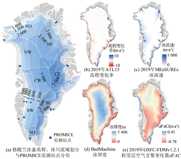
研究使用环境研究地球系统数据记录集(Making Earth System Data Records for Use in Research Environments,MEaSUREs)格陵兰冰盖年度冰流速数据产品 (Greenland Annual Ice Sheet Velocity Mosaics from SAR and Landsat, version 4,NSIDC-0725)和冰桥格陵兰厚度数据产品(IceBridge BedMachine Greenland, version 5,IDBMG4)计算冰通量散度。MEaSUREs产品基于TerraSAR-X/TanDEM-X与Sentinel-1A/B合成孔径雷达数据,以及 Landsat8光学影像数据生产,空间分辨率200 m,包括标量冰流速与垂直方向上的2个矢量冰流速,可通过美国国家冰雪数据中心(https://nsidc.org/data/nsidc-0725/versions/4)获取^[17]。IDBMG4产品结合1993—2021年MCoRDS和HiCARS等雷达数据生产,空间分辨率150 m,可通过美国国家冰雪数据中心(https://nsidc.org/data/idbmg4/versions/5)获取^[18]。在格陵兰冰盖大多数地区,冰厚度变化量与冰厚度本身相比可以忽略不计^[19],因此,本研究在研究时段内使用同一冰厚度数据,并将冰流速与冰厚度数据通过双线性内插法重采样为1 km(图1(c)—(d))。

研究使用粒雪密实化模型GSFC-FDMv1.2.1输出的粒雪层空气含量(firn air content,FAC),将冰盖高程变化转换为质量变化。数据可在欧洲开放存储库Zenodo(https://zenodo.org/record/7221954#.Y27_wXZBzb1)获取^[20]。研究利用每5 d一期12.5 km空间分辨率的GSFC-FDMv1.2.1数据,选择最接近高程变化测算时间的FAC计算年际粒雪层空气含量dFAC,并通过双线性内插法重采样至1 km(图1(e))。

研究使用RACMO和MAR 2种常用的区域气候模型(regional climate model,RCM)获取SMB模拟结果进行对比分析。RACMO提供1 km空间分辨率的SMB数据,MAR的空间分辨率为6.5 km,研究采用双线性内插法重采样至5 km。研究使用格陵兰冰盖监测计划(programme for monitoring of the Greenland ice sheet,PROMICE)站点提供的SMB实测数据作为验证数据。该数据由丹麦地质调查局提供(https://promice.org)^[21],包含自1892年以来格陵兰冰盖消融区46个站点大约3 000个SMB的测量值,每个测量值都附有位置、日期、数据质量等信息(图1(a))。

2 研究方法

2.1 格陵兰冰盖SMB估算总体流程

格陵兰冰盖MB对应的冰盖高程变化(h_MB)受到SMB,D,冰盖底部物质平衡(basal mass balance,BMB)和基岩垂直运动(vertical bedrock,VB)(冰期回弹等)等因素影响(对应的高程变化分别为 $h_{S M B}, h_{D}$ ,h_BMB,h_VB)^[14]。其中,除h_D外,均以高程增加为正,高程下降为负,因为D代表溢出冰川崩解造成的高程变化,故排出导致的高程降低为正,流入导致的高程上升为负,符号与其他变量相反。计算公式为:

(1)h_MB=h_SMB-h_D+h_BMB+h_VB。

在研究时段内,BMB相对MB占比很小,VB变化不大,因此可以忽略不计^[22-23],得到简化公式为:

(2)h_MB=h_SMB-h_D,

(3)h_SMB=h_MB+h_D=d_H+▽q,

式中: d_H为某一时段内观测到的冰盖高程变化; ▽q为该时段内封闭体积内由冰通量引起的冰盖高程变化,这里将之定义为冰通量散度,作为标量其正负含义与h_D一致。

SMB是高度变化量与冰雪密度ρ的乘积,计算公式为:

(4)SMB=(d_H+▽q)·ρ 。

由于粒雪密实化作用,冰面不同地点与深度的冰雪密度不同^[24]。若均采用固定密度值,会造成SMB估算的较大误差^[25]。为此,研究选择去除单位面积内以深度表示的FAC,即假定将粒雪层全部压实为冰,再统一使用冰密度ρ_ice=917 kg·m^-3估算SMB,公式为:

(5)SMB=(d_H+▽q-d_FAC)·ρ_ice,

式中d_FAC为FAC变化量。由上式可知,估算冰盖表面质量平衡SMB需要具有同一时段内的冰盖高程变化量d_H、冰通量散度▽q和FAC变化量d_FAC。冰通量散度(ice flux divergence, ▽q)是反映单位时段封闭体积内冰通量(ice flux, q)大小的标量,描述了冰通量的密度,正值表示发散,负值表示吸收。

2.2 基于像元的冰通量散度有限差分估算方法

研究采用基于像元的有限差分方法^[26]估算格陵兰冰盖各像元的冰通量散度。计算时,可将冰通量(矢量)分解为相互垂直的2个方向^[27],并进一步表示为冰通量在2个方向上的梯度和,公式为:

(6)

▽ q = ▽ (q_{x} + q_{y}) = \frac{\partial q_{x}}{\partial x} + \frac{\partial q_{y}}{\partial y} 。

冰通量是一个雪柱内从冰盖底部到表面的各层冰流速在垂直方向上的积分^[28],可表示为该雪柱冰流速的平均值与该处冰厚度的乘积。冰层内冰流速的平均值一般较难获取,可利用冰层内冰流速平均值与冰盖表面流速的经验比值F近似表示。一般来说,冰体蠕变指数取n=3,此时F介于0.8~1之间^[28]。若冰体受内部形变控制且完全没有基底滑动,F=0.8; 若全为基底滑动控制,则F=1。F在格陵兰冰盖不同地区并不相同^[29],在冰川内陆地区冰盖与基岩几乎无相对滑动的区域F较小,而冰川边缘F较大^[30-31]。Meierbachtol等^[32]认为冰盖边缘向内陆50 km内的区域冰下水系发达,基底滑动显著,因此,研究将距离冰盖边缘50 km内的区域F设定为0.9,而内陆其他区域F设定为0.8。冰通量q的计算公式为:

(7)

q = \int_{B}^{S} u (z) d z = \bar{u} H = F u s H,

式中: B为冰川基底; S为冰川表面; u(z)为冰川内部每一层的冰流速; $\bar{u}$ 为从冰川基底到冰川表面的冰层内冰流速平均值; H为冰川基底到冰川表面的冰厚度; u_s为冰盖表面流速。对冰盖表面流速进行矢量分解,u_s=u_s(u,v)。再将x,y方向的冰通量代入式(7),可进一步表示为:

(8)

▽ q = F [\frac{\partial (u H)}{\partial x} + \frac{\partial (v H)}{\partial y}] = F (u \frac{\partial H}{\partial x} + v \frac{\partial H}{\partial y} + H \frac{\partial u}{\partial x} + H \frac{\partial v}{\partial y}) 。

计算▽q需要获取各像元冰流速、冰厚度及二者在x与y方向上的梯度值,可将梯度微分值近似为有限差分值,公式为:

(9)

{(\frac{\partial H}{\partial x})}_{i} = \frac{H (i + 1) - H (i - 1)}{2 r} 。

式中: r为相关系数; i为分量; 冰厚度和冰流速数据的误差在有限差分中会被放大^[27]。因此,在各分量分别有限差分计算时和各分量累加后,参考Van Tricht等^[23]研究使用自适应窗口大小的高斯低通滤波进行平滑处理。滤波的窗口大小随窗口中心像元的冰厚度而自适应改变,研究将高斯滤波参数σ设置为中心像元冰厚度的20倍。为防止平滑过程对冰通量总量造成影响,平滑完成后按照未平滑时的冰通量总和与平滑后的冰通量总和的比值进行等比例放缩,得到满足通量总量与实测数据一致的各像元冰通量散度。

此外,冰流速误差较大和冰流速本身较大的区域在进行差分计算时会显著放大测量误差,即

(10)

{σ_{▽ q}}^{2} = F^{2} ({(\frac{\partial H}{\partial x})}^{2} σ_{u}^{2} + u^{2} {σ_{\frac{\partial H}{\partial x}}}^{2} + {(\frac{\partial H}{\partial y})}^{2} σ_{v}^{2} + v^{2} {σ_{\frac{\partial H}{\partial y}}}^{2} + {(\frac{\partial u}{\partial x})}^{2} σ_{H}^{2} + H^{2} {σ_{\frac{\partial u}{\partial x}}}^{2} + {(\frac{\partial v}{\partial y})}^{2} σ_{H}^{2} + H^{2} {σ_{\frac{\partial v}{\partial y}}}^{2}),

式中σ_i为分量i的误差。因此,研究认为冰流速小于100 m/a且流速观测误差小于0.8 m/a的低流速冰川区^[33]的估算结果具有较高的可信度。

2.3 粒雪密实化模型估算冰盖质量变化

GSFC-FDMv1.2.1粒雪密实化模型利用全球大气再分析模型MERRA-2输出的降雪、总降水、蒸发和气温等变量,通过实测剖面数据校准模型运转过程,输出粒雪层密度与FAC数据集^[34]。FAC反映单位面积冰面至冰盖内部达到冰密度的深度所对应的粒雪柱中包含空气的体积,即当粒雪柱被压缩到冰密度时发生的厚度变化^[35]。因此,在冰盖高程变化中去除FAC对应的高程变化后,即可采用冰密度(ρ_ice=917 kg·m^-3)估算冰盖质量变化。

2.4 SMB估算结果对比分析

研究通过均方根误差(root mean square error,RMSE)与相关系数(correlation coefficient,r)分析SMB估算误差。首先对比分析本研究遥感估算SMB,RCM模拟SMB与PROMICE实测SMB,由于PROMICE 2020年232_SCO_L站点为冰盖外围像元,且该站点PROMICE实测数据与MAR模拟SMB以及本研究遥感估算SMB均有大于2.69 m w.e.·a^-1的显著差异,因此判定其为异常值并剔除,其余2019年与2020年研究区范围内的PROMICE站点数据均保留。进一步,将本研究遥感估算SMB结果重采样到5 km,与MAR和RACMO模型SMB模拟结果对比分析。

3 结果与分析

研究估算得到2019年与2020年1 km空间分辨率的格陵兰冰盖表面物质平衡空间分布(图2)。2019年SMB估算范围占总冰盖面积的79.7%,2020年SMB估算范围占总冰盖面积的81.6%,剩余18.4%~20.3%的区域由于冰流速过大或冰流速测量误差过大并未估算SMB。整体来看,2019年与2020年SMB估算结果在北部NO流域、东北NE流域、东南SE流域和西南SW流域的缺失区域类似(面积百分比差值小于0.62%),在东部CE流域和西部CW流域缺失区域则有较为明显的差异(面积百分比差值大于4.52%)。在北部NO流域,SMB估算缺失区域非常小(面积百分比小于6%),而南部SO流域缺失区域非常大(面积百分比大于45%)。整体来看,研究获得了格陵兰80%区域的SMB估算结果。

图2

图2 冰盖表面物质平衡SMB遥感估算结果

Fig.2 SMB remote sensing estimation results

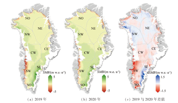
2019年与2020年格陵兰冰盖SMB整体空间分布较为一致,冰盖西南SW流域在2 a内均为表面物质高损失区(SMB均值<0.19 m w.e.·a^-1),表面物质积累在2 a内均主要集中在冰盖南部SO流域和东南SE流域,这2个流域表面物质积累量之和在2019年(1.19±1.16 m w.e.·a^-1)与2020年(1.16±0.80 m w.e.·a^-1)较为相近,冰盖北部低海拔消融区在2019年和2020这2 a内物质损失量均较高(图2)。

格陵兰冰盖2019年比2020年消融更旺盛,西南SW流域2019年的SMB均值为-0.23±1.28 m w.e.·a^-1,显著低于2020年的0.19±0.98 m w.e.·a^-1; 冰盖南部SO流域2019年的SMB(0.69±1.20 m w.e.·a^-1)同样显著低于2020年的SMB(1.15±0.95 m w.e.·a^-1)。2019年高积累区物质积累量和高损失区物质损失量都较大,表面物质高损失区西南SW流域沿海物质损失量高于2020年,而表面物质高积累区东南SE流域的内陆地区物质积累量同样高于2020年(图2),2019年各流域SMB标准差均高于2020年。可以看出,2019年总体消融旺盛,但局地仍有较高物质积累,说明暖年冰盖表面物质平衡的积累与损失更加剧烈。

研究选取16个PROMICE实测站点(图1(a))验证本研究SMB估算精度(图3)。结果表明,本研究2019年与2020年遥感估算SMB与PROMICE实测SMB的RMSE=0.519 m w.e.,小于MAR模型对应的RMSE = 0.565 m w.e.和RACMO模型对应的RMSE = 0.877 m w.e.,本研究遥感估算SMB与PROMICE实测SMB的一元线性回归模型r=0.954,略优于MAR模型对应的r=0.950,显著优于RACMO模型对应的r=0.833,且本研究遥感估算对应的回归模型拟合线斜率更接近于1。因此,本研究遥感估算SMB与PROMICE实测SMB具有较好的一致性,优于MAR和RACMO这2个RCM模拟的SMB。

图3

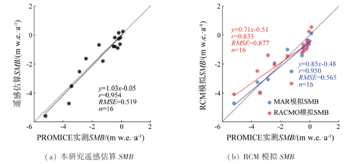
图3 与PROMICE实测SMB的对比分析

Fig.3 Comparison and analysis with PROMICE in-situ SMB observations

研究以2019年为例对比分析本研究遥感估算SMB与区域气候模型MAR和RACMO模拟SMB(图4)。遥感估算SMB与MAR模拟SMB的RMSE=0.443 m w.e.,一致性较好,对应的一元线性回归模型r=0.886。本研究遥感估算SMB与RACMO模拟SMB的RMSE=0.531 m w.e.,对应的一元线性回归模型r=0.820。因此,本研究遥感估算SMB与MAR模拟SMB结果更相近。

图4

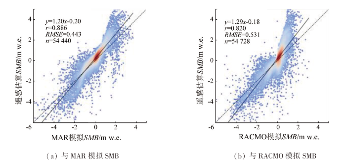
图4 2019年本研究遥感估算SMB与RCM(MAR,RACMO)模拟SMB的回归分析

Fig.4 Regression analysis of 2019 remote sensing estimated SMB in this study and RCM (MAR, RACMO) simulated SMB

研究进一步分海拔对比分析本研究遥感估算SMB与MAR和RACMO模拟的SMB(图5)。结果表明,三者反映的表面物质损失集中分布在冰盖海拔1 500 m以下,而1 500 m以上的冰盖内陆地区则有较小的表面物质积累。2种RCM模拟SMB在海拔500~1 500 m与本研究遥感估算SMB结果较为一致,但在1 500 m以上的高海拔地区RCM模拟SMB与本研究遥感估算SMB相对差异较大,RCM模拟结果低估了高海拔地区的表面物质积累。

图5

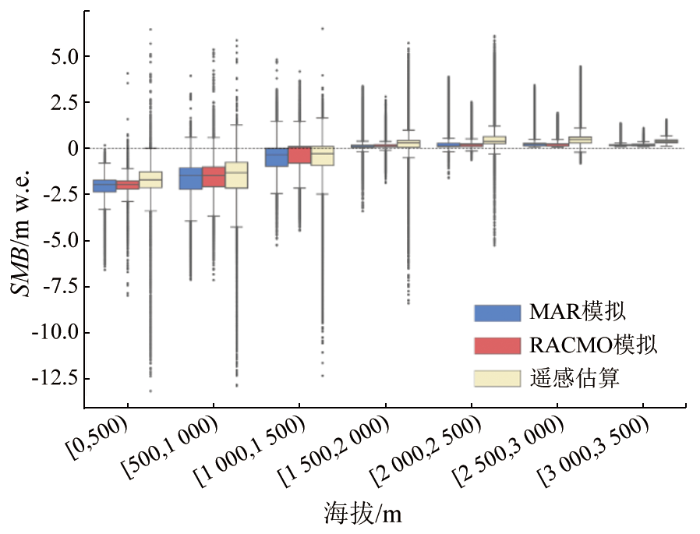
图5 本研究遥感估算SMB与RCM(MAR,RACMO)模拟SMB分海拔对比

Fig.5 Comparison between remote sensing estimated SMB in this study and RCM (MAR, RACMO) simulated SMB elevations

4 结论

研究提出了一种综合冰通量散度的格陵兰冰盖表面物质平衡遥感估算方法,估算并分析了2019年与2020年格陵兰冰盖SMB空间分布。2019年与2020年SMB估算范围占总冰盖区域80%,剩余区域由于冰流速对估算误差的影响,并未估算SMB。在2 a内,西南流域(SW)均为表面物质高损失区,南部流域(SO)和东南流域(SE)均为表面物质高积累区,北部沿海小范围在2 a内物质损失量均较高,其余大部分地区的SMB值较小。2019年与2020年相比,总体消融旺盛,但局地仍有较高物质积累。本研究遥感估算SMB与PROMICE实测SMB具有较好的一致性(RMSE为0.519 m w.e.),优于区域气候模型模拟SMB(RMSE 为 0.565~0.877 m w.e.),因而提供了一种可靠的估算格陵兰冰盖表面物质平衡空间分布的方法。

本研究显示出遥感估算格陵兰冰盖表面物质平衡的潜力,但估算结果依赖于冰厚度与冰流速数据,同时,估算结果缺少格陵兰冰盖内陆地区观测数据的验证。未来随着精度更高的多时相冰厚度与冰流速数据出现,本方法有望更精细化地估算格陵兰冰盖表面物质平衡。最后,本文提出的估算方法通过有限差分计算冰通量散度,没有反映冰面微地形对冰通量的影响,未来可探索利用三维冰流模型计算冰通量,进一步提高格陵兰冰盖冰通量与表面物质平衡的估算精度。

参考文献

原文顺序

文献年度倒序

文中引用次数倒序

被引期刊影响因子

[1]

Morlighem

, Williams

C N

, Rignot

, et al.

BedMachine v3:Complete bed topography and ocean bathymetry mapping of Greenland from multibeam echo sounding combined with mass conservation

[J]. Geophysical Research Letters, 2017, 44(21):11051-11061.

DOI:10.1002/2017GL074954 PMID:29263561 [本文引用: 1]

Greenland's bed topography is a primary control on ice flow, grounding line migration, calving dynamics, and subglacial drainage. Moreover, fjord bathymetry regulates the penetration of warm Atlantic water (AW) that rapidly melts and undercuts Greenland's marine-terminating glaciers. Here we present a new compilation of Greenland bed topography that assimilates seafloor bathymetry and ice thickness data through a mass conservation approach. A new 150 m horizontal resolution bed topography/bathymetric map of Greenland is constructed with seamless transitions at the ice/ocean interface, yielding major improvements over previous data sets, particularly in the marine-terminating sectors of northwest and southeast Greenland. Our map reveals that the total sea level potential of the Greenland ice sheet is 7.42 ± 0.05 m, which is 7 cm greater than previous estimates. Furthermore, it explains recent calving front response of numerous outlet glaciers and reveals new pathways by which AW can access glaciers with marine-based basins, thereby highlighting sectors of Greenland that are most vulnerable to future oceanic forcing.

[2]

Shepherd

, Ivins

, Rignot

, et al.

Mass balance of the Greenland Ice Sheet from 1992 to 2018

[J]. Nature, 2020, 579(7798):233-239.

[3]

Vaughan

D G

, Comiso

J C

, Allison

, et al.

Observations:Cryosphere

[J]. Climate Change, 2013, 2103:317-382.

[4]

Van den Broeke

M R

, Enderlin

E M

, Howat

I M

, et al.

On the recent contribution of the Greenland ice sheet to sea level change

[J]. The Cryosphere, 2016, 10(5):1933-1946.

[5]

Lenaerts

J T M

, Medley

, van den Broeke

M R

, et al.

Observing and modeling ice sheet surface mass balance

[J]. Reviews of Geophysics, 2019, 57(2):376-420.

DOI:10.1029/2018RG000622 PMID:31598609 [本文引用: 2]

Surface mass balance (SMB) provides mass input to the surface of the Antarctic and Greenland Ice Sheets and therefore comprises an important control on ice sheet mass balance and resulting contribution to global sea level change. As ice sheet SMB varies highly across multiple scales of space (meters to hundreds of kilometers) and time (hourly to decadal), it is notoriously challenging to observe and represent in models. In addition, SMB consists of multiple components, all of which depend on complex interactions between the atmosphere and the snow/ice surface, large-scale atmospheric circulation and ocean conditions, and ice sheet topography. In this review, we present the state-of-the-art knowledge and recent advances in ice sheet SMB observations and models, highlight current shortcomings, and propose future directions. Novel observational methods allow mapping SMB across larger areas, longer time periods, and/or at very high (subdaily) temporal frequency. As a recent observational breakthrough, cosmic ray counters provide direct estimates of SMB, circumventing the need for accurate snow density observations upon which many other techniques rely. Regional atmospheric climate models have drastically improved their simulation of ice sheet SMB in the last decade, thanks to the inclusion or improved representation of essential processes (e.g., clouds, blowing snow, and snow albedo), and by enhancing horizontal resolution (5-30 km). Future modeling efforts are required in improving Earth system models to match regional atmospheric climate model performance in simulating ice sheet SMB, and in reinforcing the efforts in developing statistical and dynamic downscaling to represent smaller-scale SMB processes.©2019. The Authors.

[6]

Hanna

, Mernild

S H

, Cappelen

, et al.

Recent warming in Greenland in a long-term instrumental (1881—2012) climatic context:I.Evaluation of surface air temperature records

[J]. Environmental Research Letters, 2012, 7(4):045404.

[7]

Ettema

, van den Broeke

M R

, van Meijgaard

, et al.

Higher surface mass balance of the Greenland ice sheet revealed by high-re-solution climate modeling

[J]. Geophysical Research Letters, 2009, 36(12):L12501.

[8]

Goelzer

, Huybrechts

, Fürst

J J

, et al.

Sensitivity of Greenland ice sheet projections to model formulations

[J]. Journal of Glaciology, 2013, 59(216):733-749.

[9]

Noël

, van de Berg

W J

, van Wessem

J M

, et al.

Modelling the climate and surface mass balance of polar ice sheets using RACMO2-Part 1:Greenland (1958—2016)

[J]. The Cryosphere, 2018, 12(3):811-831.

[10]

Fettweis

, Box

J E

, Agosta

, et al.

Reconstructions of the 1900—2015 Greenland ice sheet surface mass balance using the regional climate MAR model

[J]. The Cryosphere, 2017, 11(2):1015-1033.

[11]

Vernon

C L

, Bamber

J L

, Box

J E

, et al.

Surface mass balance mo-del intercomparison for the Greenland ice sheet

[J]. The Cryosphere, 2013, 7(2):599-614.

[12]

Fettweis

, Hofer

, Krebs-Kanzow

, et al.

GrSMBMIP:Intercomparison of the modelled 1980—2012 surface mass balance over the Greenland Ice Sheet

[J]. The Cryosphere, 2020, 14(11):3935-3958.

[13]

Kuipers

M P

, Ligtenberg

S R M

, Noël

B P Y

, et al.

Elevation change of the Greenland Ice Sheet due to surface mass balance and firn processes,1960—2014

[J]. The Cryosphere, 2015, 9(6):2009-2025.

[14]

Cooper

M G

, Smith

L C

Satellite remote sensing of the Greenland ice sheet ablation zone:A review

[J]. Remote Sensing, 2019, 11(20):2405.

[15]

Markus

, Neumann

, Martino

, et al.

The ice,cloud,and land elevation satellite-2 (ICESat-2):Science requirements,concept,and implementation

[J]. Remote Sensing of Environment, 2017, 190:260-273.

[16]

Smith

, Sutterley

, Dickinson

, et al. ATLAS/ICESat-2 L3B Gridded Antarctic and Arctic Land Ice Height Change,Version 2 [DS]. 2022.

[17]

Joughin

. MEaSUREs Greenland Annual Ice Sheet Velocity Mosaics from SAR and Landsat,Version 4 [DS]. 2022.

[18]

Morlighem

, Williams

, Rignot

, et al. IceBridge BedMachine Greenland,Version 5 [DS]. 2022.

[19]

Hamilton

G S

, Whillans

I M

Local rates of ice-sheet thickness change in Greenland

[J]. Annals of Glaciology, 2002, 35:79-83.

[20]

Medley

, Neumann

, Zwally

H J

, et al. NASA GSFC Firn Densification Model version 1.2.1 (GSFC-FDMv1.2.1) for the Greenland and Antarctic Ice Sheets:1980—2022 (1.2.1 release 2) [DS]. 2022.

[21]

Machguth

, Thomsen

H H

, Weidick

, et al.

Greenland surface mass-balance observations from the ice-sheet ablation area and local glaciers

[J]. Journal of Glaciology, 2016, 62(235):861-887.

[22]

Brinkerhoff

, Johnson

A stabilized finite element method for calculating balance velocities in ice sheets

[J]. Geoscientific Model Development, 2015, 8(5):1275-1283.

[23]

Van

Tricht L

, Huybrechts

, Van

Breedam J

, et al.

Estimating surface mass balance patterns from unoccupied aerial vehicle measurements in the ablation area of the Morteratsch-Pers glacier complex (Switzerland)

[J]. The Cryosphere, 2021, 15(9):4445-4464.

[24]

Sørensen

L S

, Simonsen

S B

, Nielsen

, et al.

Mass balance of the Greenland ice sheet (2003—2008) from ICESat data - the impact of interpolation,sampling and firn density

[J]. The Cryosphere, 2011, 5(1):173-186.

[25]

Sutterley

T C

, Velicogna

, Fettweis

, et al.

Evaluation of reconstructions of snow/Ice melt in Greenland by regional atmospheric climate models using laser altimetry data

[J]. Geophysical Research Letters, 2018, 45(16):8324-8333.

[26]

Brocq A M

, Payne

A J

, Siegert

M J

West Antarctic balance calculations:Impact of flux-routing algorithm,smoothing algorithm and topography

[J]. Computers & Geosciences, 2006, 32(10):1780-1795.

[27]

Miles

, McCarthy

, Dehecq

, et al.

Health and sustainability of glaciers in high Mountain Asia

[J]. Nature Communications, 2021, 12(1):2868.

DOI:10.1038/s41467-021-23073-4 PMID:34001875 [本文引用: 2]

Glaciers in High Mountain Asia generate meltwater that supports the water needs of 250 million people, but current knowledge of annual accumulation and ablation is limited to sparse field measurements biased in location and glacier size. Here, we present altitudinally-resolved specific mass balances (surface, internal, and basal combined) for 5527 glaciers in High Mountain Asia for 2000-2016, derived by correcting observed glacier thinning patterns for mass redistribution due to ice flow. We find that 41% of glaciers accumulated mass over less than 20% of their area, and only 60% ± 10% of regional annual ablation was compensated by accumulation. Even without 21 century warming, 21% ± 1% of ice volume will be lost by 2100 due to current climatic-geometric imbalance, representing a reduction in glacier ablation into rivers of 28% ± 1%. The ablation of glaciers in the Himalayas and Tien Shan was mostly unsustainable and ice volume in these regions will reduce by at least 30% by 2100. The most important and vulnerable glacier-fed river basins (Amu Darya, Indus, Syr Darya, Tarim Interior) were supplied with >50% sustainable glacier ablation but will see long-term reductions in ice mass and glacier meltwater supply regardless of the Karakoram Anomaly.

[28]

Cuffey

K M

, Paterson

W S B

. The Physics of Glaciers[M]. Newyork: Academic Press, 2010.

[29]

Zekollari

, Huybrechts

, Fürst

J J

, et al.

Calibration of a higher-order 3-D ice-flow model of the Morteratsch glacier complex,Engadin,Switzerland

[J]. Annals of Glaciology, 2013, 54(63):343-351.

[30]

Bons

P D

, Kleiner

, Llorens

M G

, et al.

Greenland ice sheet:Higher nonlinearity of ice flow significantly reduces estimated basal motion

[J]. Geophysical Research Letters, 2018, 45(13):6542-6548.

[31]

Reeh

, Mohr

J J

, Madsen

S N

, et al.

Three-dimensional surface velocities of Storstrømmen glacier,Greenland,derived from radar interferometry and ice-sounding radar measurements

[J]. Journal of Glaciology, 2003, 49(165):201-209.

[32]

Meierbachtol

, Harper

, Humphrey

Basal drainage system response to increasing surface melt on the greenland ice sheet

[J]. Science, 2013, 341(6147):777-779.

DOI:10.1126/science.1235905 PMID:23950535 [本文引用: 1]

Surface meltwater reaching the bed of the Greenland ice sheet imparts a fundamental control on basal motion. Sliding speed depends on ice/bed coupling, dictated by the configuration and pressure of the hydrologic drainage system. In situ observations in a four-site transect containing 23 boreholes drilled to Greenland's bed reveal basal water pressures unfavorable to water-draining conduit development extending inland beneath deep ice. This finding is supported by numerical analysis based on realistic ice sheet geometry. Slow meltback of ice walls limits conduit growth, inhibiting their capacity to transport increased discharge. Key aspects of current conceptual models for Greenland basal hydrology, derived primarily from the study of mountain glaciers, appear to be limited to a portion of the ablation zone near the ice sheet margin.

[33]

Mankoff

K D

, Colgan

, Solgaard

, et al.

Greenland Ice Sheet solid ice discharge from 1986 through 2017

[J]. Earth System Science Data, 2019, 11(2):769-786.

DOI:10.5194/essd-11-769-2019 [本文引用: 1]

We present a 1986 through 2017 estimate of Greenland Ice Sheet ice discharge. Our data include all discharging ice that flows faster than 100 m yr(-1) and are generated through an automatic and adaptable method, as opposed to conventional hand-picked gates. We position gates near the present-year termini and estimate problematic bed topography (ice thickness) values where necessary. In addition to using annual timevarying ice thickness, our time series uses velocity maps that begin with sparse spatial and temporal coverage and end with near-complete spatial coverage and 6 d updates to velocity. The 2010 through 2017 average ice discharge through the flux gates is similar to 488 +/- 49 Gt yr(-1). The 10 % uncertainty stems primarily from uncertain ice bed location (ice thickness). We attribute the similar to 50 Gt yr(-1) differences among our results and previous studies to our use of updated bed topography from BedMachine v3. Discharge is approximately steady from 1986 to 2000, increases sharply from 2000 to 2005, and then is approximately steady again. However, regional and glacier variability is more pronounced, with recent decreases at most major glaciers and in all but one region offset by increases in the NW (northwestern) region. As part of the journal's living archive option, all input data, code, and results from this study will be updated when new input data are accessible and made freely available at https://doi.org/10.22008/promice/data/ice_discharge.

[34]

Medley

, Neumann

T A

, Zwally

H J

, et al.

Simulations of firn processes over the Greenland and Antarctic ice sheets:1980—2021

[J]. The Cryosphere, 2022, 16(10):3971-4011.

[35]

Ligtenberg

S R M

, Kuipers

Munneke P

, van den Broeke

M R

Present and future variations in Antarctic firn air content

[J]. The Cryosphere, 2014, 8(5):1711-1723.