基于无人机高光谱影像的农田土壤有机碳含量估算——以湟水流域农田为例

doi:10.6046/zrzyyg.2023005

基于无人机高光谱影像的农田土壤有机碳含量估算——以湟水流域农田为例

宋奇^,¹^,²^,³, 高小红^,¹^,²^,³^,⁴, 宋玉婷¹^,²^,³, 黎巧丽¹^,²^,³, 陈真¹^,²^,³, 李润祥¹^,²^,³, 张昊¹^,²^,³, 才桑洁¹^,²^,³

1.青海师范大学地理科学学院,西宁 810008

2.青海省自然地理与环境过程重点实验室,西宁 810008

3.青藏高原地表过程与生态保育教育部重点实验室,西宁 810008

4.高原科学与可持续发展研究院,西宁 810008

Estimation of soil organic carbon content in farmland based on UAV hyperspectral images: A case study of farmland in the Huangshui River basin

SONG Qi^,¹^,²^,³, GAO Xiaohong^,¹^,²^,³^,⁴, SONG Yuting¹^,²^,³, LI Qiaoli¹^,²^,³, CHEN Zhen¹^,²^,³, LI Runxiang¹^,²^,³, ZHANG Hao¹^,²^,³, CAI Sangjie¹^,²^,³

1. School of Geographical Sciences, Qinghai Normal University, Xining 810008, China

2. Qinghai Province Key Laboratory of Physical Geography and Environmental Process, Xining 810008, China

3. MOE Key Laboratory of Tibetan Plateau Land Surface Processes and Ecological, Xining 810008, China

4. Academy of Plateau Science and Sustainability, Xining 810008, China

通讯作者: 高小红(1963-),女,博士生导师,教授,研究方向为遥感应用与地理空间数据分析。Email:xiaohonggao226@163.com。

责任编辑: 陈昊旻

收稿日期: 2023-01-3 修回日期: 2023-03-8

Received: 2023-01-3 Revised: 2023-03-8

作者简介 About authors

宋奇(1996-),男,博士研究生,研究方向为遥感应用与地理空间数据分析。Email: tarimsongqi@163.com。

摘要

快速、准确地估算农田土壤有机碳含量并对其进行空间分布制图,有利于土壤精细化管理和智慧农业的发展。该文以青海湟水流域3个典型农田区为例,在研究区内同步采集296个土壤样品和相应的野外原位光谱,使用无人机搭载高光谱相机进行影像获取,并对土壤样品进行室内光谱采集和有机碳含量测定。对光谱反射率进行7种不同形式的变换,通过相关性分析从中筛选出主要特征波段,利用多元线性回归、偏最小二乘回归和随机森林3种方法分别对室内光谱、野外原位光谱和无人机光谱进行建模,对比各模型的精度。用光谱直接转换法对无人机光谱进行校正,使用校正后的无人机光谱最优模型进行建模,模型代入无人机高光谱影像进行有机碳含量制图,最后对满足制图精度要求的农田区进行分析和讨论。结果表明: ①除对无人机高光谱进行对数变换后的多元线性回归不能估算有机碳外(相对分析误差为1.375),实验室光谱、野外原位光谱及无人机高光谱的原始光谱及所有转换方法均能对有机碳进行估算,决定系数R²为0.562~0.942,均方根误差为1.713~5.211,相对分析误差为1.445~4.182; ②在所有光谱变换方法中,多元散射校正+一阶微分变换与有机碳含量的相关性最高,特征波段分别为429~449 nm, 498~527 nm, 830~861 nm和869 nm; ③在所有建模结果中,随机森林模型精度最高,其次为偏最小二乘模型,多元线性回归模型精度最低,校正后的无人机光谱建模精度均有所提高; ④3个农田区的反演精度均满足制图要求,R²均在0.88以上。其中,A农田区有机碳含量均值最高,为28.88 g·kg^-1,整体空间分布均匀; B农田区均值为13.52 g·kg^-1,整体分布呈现出较强的空间差异性; C农田区有机碳含量均值最低,为8.54 g·kg^-1,高值和低值的分化明显。本研究可为无人机高光谱遥感技术应用于田间尺度的土壤有机碳含量估算和数字制图提供参考。

关键词： 无人机; 高光谱遥感; 土壤有机碳; 光谱特征选择; 光谱校正

Abstract

Rapid and accurate estimation and spatial distribution mapping of soil organic carbon content in farmland facilitate the refined management of soil and the development of smart agriculture. This study investigated three typical farmland areas in the Huangshui River basin of Qinghai Province using 296 soil samples and corresponding field in situ spectra collected synchronously. The unmanned aerial vehicle (UAV) with a hyperspectral camera was employed for image acquisition, and the soil samples were tested for spectral acquisition and organic carbon content in the laboratory. The spectral reflectance was transformed into seven different forms, and the main characteristic bands were screened out through correlation analysis. Using multiple linear regression, partial least squares regression, and random forest, the experimental spectra, field in situ spectra, and UAV spectra were modeled, with the accuracy of the models compared. The UAV spectra were corrected using the direct spectral conversion method, and the optimal model of corrected UAV spectra was used for modeling. The model was substituted into the UAV hyperspectral images for the organic carbon content mapping. Finally, the farmland areas meeting the mapping accuracy requirements were analyzed and discussed. The results show that: ① The multiple linear regression after logarithmic transformation of UAV hyperspectra failed to estimate the organic carbon content, with a relative percent deviation (RPD) of 1.375. Except for it, the experimental spectra, field in situ spectra, and original spectra of UAV hyperspectra as well as all conversion methods could estimate the organic carbon content, with coefficients of determination (R²) ranging from 0.562 to 0.942, root mean square errors (RMSEs) ranging from 1.713 to 5.211. and RPDs between 1.445 and 4.182; ② Among all spectral transformation methods, multiple scatter correction and first-order differential transformation exhibited the highest correlation with the organic carbon content, presenting characteristic bands of 429~449 nm, 498~527 nm, 830~861 nm, and 869 nm; ③ As revealed by the modeling results, the random forest model manifested the highest accuracy, followed by the partial least squares model and the multiple linear regression model in turn. The corrected UAV spectra yielded improved modeling accuracy; ④ The inversion accuracy of the three farmland areas all met the mapping requirements, with R² values above 0.88. Farmland A exhibited the highest average organic carbon content of 28.88 g·kg^-1 and an overall uniform spatial distribution. Farmland B manifested average organic carbon content of 13.52 g·kg^-1 and a significantly varying spatial distribution. Farmland C displayed the lowest average organic carbon content of 8.54 g·kg^-1 and significant differentiation between high and low values. This study can be referenced for the application of UAV hyperspectral remote sensing technology to the field-scale estimation and digital mapping of soil organic carbon content.

Keywords： unmanned aerial vehicle (UAV); hyperspectral remote sensing; soil organic carbon; spectral feature selection; spectrum correction

PDF (17204KB) 元数据多维度评价相关文章导出 EndNote| Ris| Bibtex 收藏本文

本文引用格式

宋奇, 高小红, 宋玉婷, 黎巧丽, 陈真, 李润祥, 张昊, 才桑洁. 基于无人机高光谱影像的农田土壤有机碳含量估算——以湟水流域农田为例[J]. 自然资源遥感, 2024, 36(2): 160-172 doi:10.6046/zrzyyg.2023005

SONG Qi, GAO Xiaohong, SONG Yuting, LI Qiaoli, CHEN Zhen, LI Runxiang, ZHANG Hao, CAI Sangjie. Estimation of soil organic carbon content in farmland based on UAV hyperspectral images: A case study of farmland in the Huangshui River basin[J]. Remote Sensing for Land & Resources, 2024, 36(2): 160-172 doi:10.6046/zrzyyg.2023005

0 引言

土壤有机碳(soil organic carbon,SOC)作为土壤碳库的重要组成部分,估算其含量变化对作物生长和农业生产具有重要意义^[1]。SOC含量也是土壤质量和肥力的重要指标,对有机碳含量进行空间分布制图可为实现精准农业管理和施肥提供重要参考信息,从而提高田间管理水平^[2]。因此,亟需对田间尺度的SOC空间分布特征进行高精度的量化与监测。

传统测定SOC含量的方法是野外采集土壤样品,通过实验室化学分析得到SOC含量^[3]。这样的方式费时、费力、经济成本高、监测结果具有滞后性,并且由此获取的SOC数据通常是密度较低的点状数据,难以满足SOC空间分布快速可视化的要求^[4]。因此,快速准确地监测并及时掌握农田SOC含量及空间分布情况,对提高耕地质量和土地利用效率非常重要。运用无人机高光谱遥感技术对农田SOC含量进行估算并制图,不仅使得数据获取更加实时便捷,而且拥有较高的空间分辨率和光谱分辨率,进一步为精准农业提供科学方案^[5]。

近年来,将无人机高光谱遥感技术应用于土壤属性的估算研究已越来越多。Hu等^[6]利用无人机高光谱遥感技术估算田间土壤盐分含量并绘制土壤盐分空间分布图; Sankey等^[7]利用无人机高光谱遥感技术对小尺度的牧场SOC含量进行了估算; Ge等^[8]将无人机高光谱影像用于估算新疆维吾尔自治区典型农业区的土壤含水量; 王敬哲等^[9]将无人机高光谱数据进行不同的数学变换,在筛选出最优变换方式后,构建干旱区绿洲农田土壤含水量的定量估算模型; 祝元丽等^[10]运用无人机高光谱数据对中国东北黑土和比利时黄土进行了SOC含量的反演。然而,将无人机高光谱遥感技术应用于流域范围的研究很少,并且大部分无人机高光谱土壤属性估算研究的实地采样点较少,难以验证其准确性。此外,对多块农田、不同翻耕和冬灌阶段的田间SOC含量进行空间分布制图的研究鲜见报道。

由于土壤水分的影响,光谱中存在大量的干扰信息,直接影响SOC含量估算的精度。如何有效去除土壤水分含量的影响,是土壤属性预测所面临的难题^[11]。为了消除土壤水分因素的干扰,获取更多有效的光谱信息,广大学者提出了多种方法来提高SOC的估算精度。洪永胜等^[12]运用外部参数正交化法(external parameters orthogonalization, EPO)进行土壤水分校正,该算法将偏最小二乘回归(partial least squares regression, PLSR)模型的预测偏差比提升了0.6; Hu等^[13]分别运用光谱直接转换法(direct standardization, DS)、分段直接转换法(piecewise direct standardization, PDS)、广义最小二乘加权法(general least squares weighting, GLSW)和正交信号处理法(orthogonal signal correction, OSC)对高光谱进行土壤水分去除,结果表明DS的校正结果最佳; Ji等^[14]运用DS算法对浙江水稻田土壤进行光谱校正,其中PLSR模型精度R²提升了0.44,相对分析误差(relative percent deviation,RPD)提升了1.26,表明DS算法能很好地去除水分对光谱的影响。因此,本文拟采用DS算法对无人机光谱进行水分校正,以提高估算模型的精度。

本文以青海湟水流域3个收割后和春播前的典型农田区为例,对田间土壤进行样品采集并测定野外土壤原位光谱,同期获取无人机高光谱影像,利用多元线性回归、偏最小二乘回归和随机森林3种建模方法分别对实验室光谱、野外光谱和无人机高光谱进行建模,探索无人机高光谱遥感估算农田土壤SOC的能力,并在此基础上进行SOC制图,为农田土壤精细化管理和智慧农业的发展提供数据支持。

1 研究区概况及数据源

1.1 研究区概况

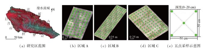
研究区位于青海湟水流域(E100° 42'~103° 04',N36° 02'~37° 28'),如图1(a)所示,地处黄土高原向青藏高原的过渡地带。流域内气候属于高原干旱、半干旱大陆性气候,日照充足,昼夜温差变化大,年均气温为2.5~7.5 ℃^[15]。在研究区内选定3个典型农田区为试验区(图1(b)—(d)),其中A区面积为2 hm²,长宽分别为200 m×100 m,土壤类型为黑钙土,作物类型为燕麦,采样时还未进行翻地,内有少量麦茬和秸秆; B区面积为4 hm²,长宽分别为400 m×100 m,土壤类型为黑钙土,作物类型为油菜,采样时已翻地,内无麦茬和秸秆; C区面积为3.36 hm²,长宽分别为240 m×140 m,土壤类型为栗钙土,作物类型为土豆和玉米,咨询当地农民得知采样时已翻地并且在2021年10月初收割后进行了冬灌,内无麦茬和秸秆。采用五点采样法采集土壤样本(图1(e))。

图1

新窗口打开| 下载原图ZIP| 生成PPT

图1 研究区位置及采样点分布

Fig.1 Location of the study area and sampling points

1.2 土壤样品采集与无人机影像获取

1.2.1 野外原位土壤光谱与田间土壤样品采集

2021年9月21日收割后、2022年3月23—25日和27—28日播种前分别在A区、B区和C区内按20 m×20 m的网格进行布点,去除采样点表面的庄稼残留物、石块等杂物后,将土壤表面抚平整。从C区冬灌到正式采样有近半年时间,此期间C区无人为活动,正式采样时,C区土壤较为干燥,3个区域无明显的土壤水分差异。首先使用美国ASD FieldSpec 4型(350~2 500 nm)地物光谱仪采集样点野外原位土壤光谱数据,光纤距离地面15 cm,在东西南北4个方向各测5条光谱,每个样点共测定20条光谱。随后采集样点0~20 cm深度的土壤,约2 kg,混合均匀装入密封带内,同时GPS记录每个采样点的坐标信息,依次完成试验区内所有样点的采集任务,最终采集土样: A区66个,B区126个,C区104个,共计296个。将所有土样在室内自然风干后,剔除杂质并研磨,先过2 mm筛,用于后期室内光谱的测定; 之后过0.15 mm筛,采用德国Elementar公司的Vario系列元素分析仪测定SOC含量^[16]。

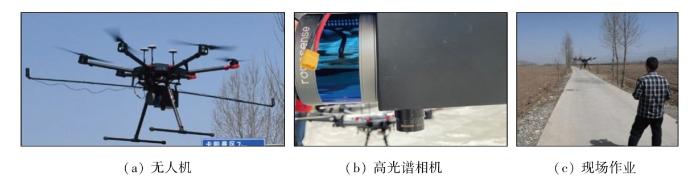
1.2.2 无人机飞行及高光谱影像获取

以大疆公司的M600 Pro无人机为平台,搭载Vis-Near (400~1 000 nm)高光谱相机(型号为Resonon Pika L, 产地为美国),分别于2021年9月21日、2022年3月23日和27日在A区、B区和C区,进行野外原位光谱、土壤采样时,同步无人机飞行拍摄田间土壤高光谱图像(图2)。无人机飞行时段为10∶00—15∶00,飞行时天气晴朗无云,风力小于3级,地表无积雪覆盖。飞行高度设置为150 m,飞行速度为4.3 m/s,图像空间分辨率为4.98 cm,获取的影像波长范围为400~1 000 nm。

图2

新窗口打开| 下载原图ZIP| 生成PPT

图2 无人机高光谱系统

Fig.2 Hyperspectral systems for unmanned aerial vehicles

1.3 数据处理

1.3.1 无人机高光谱影像预处理

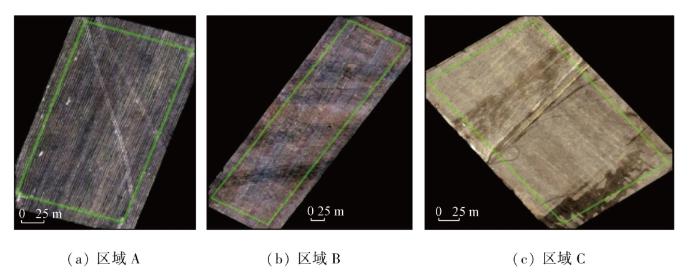
高光谱影像的处理步骤为: 首先,利用Sbgcenter对获取的高光谱影像进行航线查看和航线数据的导出,采用Omap进行航线边界分割,去除起飞和降落的无效航线; 然后基于AirlineDivision (机载高光谱切割)对高光谱数据进行预分割; 再利用MegaCube进行辐射定标和大气校正,分别利用ArcGIS和ENVI对影像进行地理配准(参考数据是无人机自带的RPC文件及其拍摄的正射底图)及配准后影像的拼接; 最后,利用MegaCube制作影像超立方体,在ENVI平台将超立方体转为高光谱影像,从无人机高光谱影像中提取出所有样点相对应的光谱反射率曲线,用提取的无人机光谱进行后续建模分析。A区因为地面有少量的麦茬和秸秆导致出现少量的混合像元问题,本文利用MATLAB并使用混合像元分解方法解决这种问题。先评估端元数目(有几种混合物质或元素,在此研究仅分为2类,即裸土和非裸土,使用最小误差高光谱信号辨识算法完成); 再对端元光谱进行提取(识别出裸土和非裸土,使用纯净像元指数(pure pixel index,PPI)进行提取); 最后对端元含量进行反演(计算每种端元所占的比例,在此使用全约束最小二乘算法进行计算)。最终处理后的影像如图3所示。

图3

新窗口打开| 下载原图ZIP| 生成PPT

图3 处理后的高光谱影像

Fig.3 Hyperspectral image after processing

1.3.2 土壤室内光谱测定与预处理

测量室内土壤光谱时,为了减少外界环境对测定结果的影响,将已剔除杂质并过2 mm筛的土样放置于半径5 cm,深度1.5 cm且内部涂黑的盛样器皿中,使用ASD FieldSpec 4型地物光谱仪以及配套的高密度反射探头测定土壤光谱数据,每个土样测量20条光谱,取其平均值作为该样品的光谱数据。为保证数据的准确性,每测完一个土样立即清理手柄镜面,并且每隔20 min进行一次白板校正。使用光谱仪自带的ViewSpecPro软件进行“陡坎”校正和求平均,然后导出数据以便后续分析使用。

1.3.3 实验室有机碳成分测试与统计分析

实验室测定SOC含量的步骤为: 首先,把过0.15 mm的土样加10 %的盐酸熏蒸12 h,用以除去土样中的无机碳; 其次,用虹吸法去除盐酸上清液,随后反复加纯水、静置后去除上清液,目的是将其pH值调为中性; 最后,将样品放入烘箱6~8 h烘干,将烘干后的土样用专用锡舟包样,然后上机测试。为保证数据的准确性,每4个样品设置1个平行样,本文共296个样品,测定74个平行样。测定结果如表1所示,3个农田区SOC含量均值的大小关系为: A区>B区>C区,各农田区的变异系数为9.31~17.5 %,属于中等变异; 偏度为0.13~0.54,峰度为-1.32~1.51,满足正态分布。

表1 SOC描述性统计

Tab.1 Descriptive statistics of soil organic carbon

采样区域	样本数	最大值/(g·kg^-1)	最小值/(g·kg^-1)	平均值/(g·kg^-1)	标准差/(g·kg^-1)	变异系数/%	偏度	峰度
A区	66	33.35	22.88	28.38	2.84	10.01	0.13	-1.32
B区	126	17.48	11.13	13.75	1.28	9.31	0.54	0.39
C区	104	14.36	4.79	8.63	1.51	17.50	0.49	1.51

新窗口打开| 下载CSV

1.4 光谱处理及数学变换

由于ASD FieldSpec 4地物光谱仪测定的土壤光谱数据波长范围及光谱分辨率,与无人机高光谱数据不同,为保持光谱数据范围的一致性,将室内光谱和野外原位光谱数据进行重采样并仅保留与无人机光谱相同的400~1 000 nm波段,波段数为150个,最终确保地物光谱仪与无人机的光谱中心波段位置相同,同时去除主要水分吸收位置(900 nm)附近的光谱波段。

对数据进行处理,光谱变换公式如表2所示。

表2 光谱数学变换

Tab.2 Methods of spectral transformation

光谱数学变换	公式	描述
1/R	$1 / R_{i}$	式中: $i$ 为波长; $Δ i$ 为波长间隔; $R_{i}$ 为波长 $i$ 的光谱反射率; m和b分别为各样品光谱与平均光谱进行一元线性回归后得到的相对偏移系数和平移量; $R_{i + Δ i}$ 为与 $R_{i}$ 间隔 $Δ i$ 的光谱反射率; $R'_{i}$ 为波长 $i$ 的一阶微分光谱; $R'_{i + Δ i}$ 为与 $R_{i}$ 间隔 $Δ i$ 的一阶微分光谱; $A$ 为所有样品的原始光谱在各个波长点处求平均值所得到的平均光谱矢量; $A_{i}$ 为1×p维矩阵,表示单个样品的光谱矢量; $R_{i, M S C}$ 为第 $i$ 个样品的多元散射校正结果; ${\bar{R}}_{i}$ 为标准光谱; $i$ =1, 2, $\dots$ , $n; n$ 为样品数
lgR	lg $R_{i}$
FDR	$(R_{i + Δ i} - R_{i}) / Δ i$
SDR	$(R'_{i + Δ i} - R'_{i}) / Δ i$
MSC	$\bar{R_{i}} = \frac{\overset{n}{\sum_{i = 1}} R_{i}}{n}$
	$A_{i} = m_{i} \bar{R_{i}} + b_{i}$
	$R_{i, M S C} = \frac{(A_{i} - b_{i})}{m_{i}}$
MSC+FDR MSC+SDR	$R_{i, M S C}$ + $(R_{i + Δ i} - R_{i}) / Δ i$ $R_{i, M S C}$ + $(R'_{i + Δ i} - R'_{i}) / Δ i$

新窗口打开| 下载CSV

采用Savitzky-Golay 7点加权移动平均法对所有光谱数据进行平滑降噪处理,在此基础上进一步对光谱进行倒数1/R、对数lgR、一阶微分FDR、二阶微分SDR、多元散射校正MSC、多元散射校正MSC+一阶微分FDR和多元散射校正MSC+二阶微分SDR 这7种不同的光谱数据变换以增强特征波段信息^[17]。

将经过上述7种光谱变换后的光谱数据与SOC含量进行相关性分析,从中筛选出相关性最高的光谱变换方法和主要特征波段,用作后续土壤光谱建模。

2 研究方法

2.1 DS原理

为了消除水分含量对土壤光谱的影响,DS法、PDS法和OSC法等多被用于校正光谱。其中, DS法可以用来将野外环境下获得的土壤光谱“转换”到室内环境下获得的光谱,通过对差值光谱(无人机光谱与室内光谱的差值)的分析,建立两者的相关关系,实现环境影响因素的去除,从而进行无人机光谱校正^[18]。DS法存在如下关系,即

(1)

X_{L (h \times p)} = X_{F (h \times p)} B + k d_{s}^{t}

式中: $X_{L (h \times p)}$ 为转换样本的室内光谱数据; $h$ 为转换样本数,采用Kennard-Stone法选取最佳转换样本数; $p$ 为光谱波段数; $X_{F (h \times p)}$ 为转换样本的无人机光谱数据; $B$ 为转换矩阵,用以衡量 $X_{L (h \times p)}$ 与 $X_{F (h \times p)}$ 之间的差异; $k d_{s}^{t}$ 为残差矩阵,用以校正无人机光谱不同于室内光谱所产生的基线偏移。同理,若需用野外原位光谱对无人机光谱进行校正,则将通过分析野外原位光谱与无人机光谱的差值,由此建立函数关系,从而实现基于野外原位光谱的无人机光谱校正。本文分别用室内光谱和野外原位光谱对无人机光谱进行校正,比较两者的校正结果,选择最优校正方法。

2.2 建模方法及评价指标

本文建模方法采用多元线性回归(multiple linear regression,MLR)、偏最小二乘回归(partial least squares regression,PLSR)和随机森林(random forest,RF)3种方法。MLR也称作逆最小二乘法,运用最小二乘法对光谱矩阵进行估计,可以有效避免关键信息的丢失; PLSR能对光谱数据进行综合性分析,解决数据间多重共线性问题,是一种经典的建模方法; RF通过建立回归树进行有效决策,稳定性高,数据适应能力强且不产生过拟合^[19]。

模型评价采用决定系数R²、均方根误差(root mean square error,RMSE)和RPD 3个指标^[20]。R²越接近于1,说明模型精度越高。RMSE越小,说明预测值与真实值越接近,模型精度越高。依据Chang等^[21]对RPD划分的等级可知,当预测模型的RPD≥2时,模型有较好的估算能力; 当1.4≤RPD<2时,该模型只能进行粗略估算; 当RPD<1.4时,表明模型的预测能力很差,不能估算。

建模之前,利用主成分分析^[22]将异常值进行剔除,共17个异常值,剩下279个样品采用浓度梯度法将SOC含量从低到高排序,按2∶1比例组成建模集(186个样本)和验证集(93个样本),每组样本的第一个和第三个为建模集,第二个样本为验证集,建模集的SOC含量范围(4.79~33.1 g·kg^-1)完全包含了验证集的含量范围(5.49~32.88 g·kg^-1),以保证验证集的SOC含量不会超出模型的量程。这种样本划分方法避免了过多的“特殊”样本被划分到建模集,最终模型能够更好地预测未知样本。由于这3个区域的采样点位置不同,单个区域的采样数较少,土壤类型单一,总体缺乏代表性,因此对3个区域进行全局建模,得到稳定的模型从而进行无人机高光谱反演。

3 结果与分析

3.1 SOC含量分级光谱特征分析

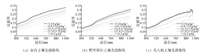
根据全国第二次土壤普查中对土壤养分含量的分级标准^[23]可知,将SOC分为5个等级,分别是等级I (>23.2 g·kg^-1)、等级II (17.4,23.2] g·kg^-1、等级III (11.6,17.4] g·kg^-1 、等级IV (5.8,11.6] g·kg^-1和等级V (≤5.8 g·kg^-1)。图4是根据每个等级的平均反射率分别得到土壤室内、野外原位以及无人机影像光谱的反射率曲线。从图4中可知,不同SOC含量的光谱曲线变化规律和曲线形态基本一致,整体呈上升趋势,反射率值的变化范围为0~0.33之间且随着SOC含量的增加而降低,呈现出负相关的关系。虽然3种光谱曲线一致,但在波长为400 nm,SOC含量≤5.8 g·kg^-1时,反射率值有所不同,野外光谱与无人机光谱均低于实验室光谱。在波长420 nm和900 nm附近,无人机光谱受系统性能和水汽因素的影响,出现明显的吸收谷。

图4

新窗口打开| 下载原图ZIP| 生成PPT

图4 各等级的SOC含量光谱曲线

Fig.4 Spectral curves of SOC content of each grade

3.2 相关分析与特征波段选择

为了减少光谱数据的冗余,挑选特征波段或敏感波段进行建模是非常必要的。利用原始室内光谱以及经过7种不同数学变换的土壤光谱曲线与实测SOC含量进行相关性分析,得到光谱与SOC含量的相关系数(图5),并从中筛选出主要特征波段(表3)。从图5可知,反射率R与SOC含量主要呈负相关,相关系数曲线呈上升趋势,最大相关系数为-0.82。1/R与SOC含量呈正相关,随着波长的增加相关系数逐渐减小。lgR与SOC的变化规律同原始光谱的变化形式相似,即呈负相关。

图5

新窗口打开| 下载原图ZIP| 生成PPT

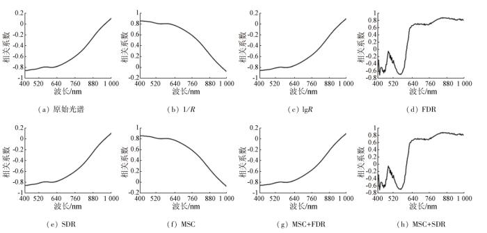
图5 SOC和不同光谱变换形式的相关性分析

Fig.5 Correlation of SOC and different spectral transformations

表3 不同光谱变换下的有机碳特征响应波段

Tab.3 Characteristic response bands of SOC under different spectral transformations

光谱反射率及各种光谱变换方法	主要特征波段/nm	特征波段数量	最大相关性波段/nm	最大相关系数
R	400~708	78	400	-0.86^*
1/R	400~598	51	412	0.85^*
lgR	400~602	52	400	-0.86^*
FDR	799~990	50	847	0.88^*
SDR	412, 449, 523, 540, 565, 590, 644, 653, 666, 713, 756, 782, 786, 804, 852, 887~949	31	786	0.44^*
MSC	400~437, 581~821	71	606	-0.89^*
MSC+FDR^①	429~449, 498~527, 830~861, 869	23	847	0.91^*
MSC+SDR	408~412, 421, 429, 433, 449, 523, 540, 556~565, 573~581, 594, 704, 786, 830, 920~949	26	565	0.56^*

①加粗为相关性最高的光谱变换方式; *为显著性水平符号。

新窗口打开| 下载CSV

FDR与SOC的相关性随着波长的增加相关性表现更为复杂,在570 nm处相关性的增幅最大。SDR与SOC的相关性变化波动很大,但整体相关系数不高,最大相关系数只有0.44。MSC与SOC含量的相关系数曲线在400~520 nm区间呈平缓下降,但在520~550 nm区间却呈直线式下降后又呈平缓上升。原始光谱经MSC+FDR变换后,SOC和反射率数据相关系数最高,最大相关系数达到0.91,是相关系数最高的光谱变换形式,主要特征波段为429~449 nm, 498~527 nm, 830~861 nm和869 nm,共计23个特征波段。MSC+SDR与SOC的相关性波动较大,相关系数曲线呈现出锯齿状的变化特征。

3.3 基于MLR,PLSR及RF的建模结果对比

野外光谱和无人机光谱所选用的特征波段位置与实验室光谱相同,分别运用MLR,PLSR及RF这3种模型对实验室光谱、野外光谱和无人机影像光谱及其各自相应的7种光谱变换所选择的特征波段与SOC含量数据建立统计关系,结果如图6所示。在室内光谱的3种建模结果中,整体建模精度较高,其中基于MSC+FDR变换后的RF建模精度最高,建模集 $R_{c a l}^{2}$ 为0.942,验证集 $R_{v a l}^{2}$ 为0.938,表明模型对SOC有很好的估算能力。在野外原位光谱的3种建模结果中,同样,也是基于MSC+FDR变换的建模精度最高,该变换方式在MLR中建模集 $R_{c a l}^{2}$ 为0.753,在PLSR中 $R_{c a l}^{2}$ 为0.834,在RF中 $R_{c a l}^{2}$ 为0.854,说明建模效果较好。无人机光谱的3种建模结果,与实验室光谱和野外原位光谱表现出一致的结果,即MSC+FDR变换形式的建模集和验证集R²为同组最高,MLR,PLSR以及RF模型的 $R_{c a l}^{2}$ 分别为0.704,0.756和0.804,整体建模精度均低于野外原位光谱和实验室光谱。综上可知,在所有光谱变换方法中,MSC+FDR变换的整体建模精度最高。在3种模型中,RF的整体建模精度最高,其次是PLSR和MLR。在3种光谱类型中,室内光谱的整体建模精度最高,其次是野外原位光谱,无人机光谱的整体建模精度最低。

图6

新窗口打开| 下载原图ZIP| 生成PPT

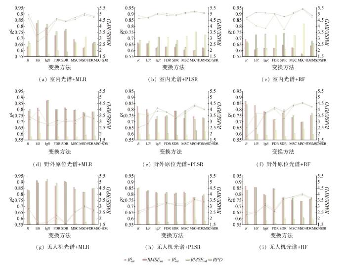
图6 室内光谱、野外原位光谱和无人机光谱的不同模型精度对比

Fig.6 Accuracies comparison of different models for indoor spectrum, field in-situ spectrum and UAV spectrum

3.4 基于校正后的无人机光谱建模

为提高无人机光谱的建模精度,分别将室内光谱和野外原位光谱作为参照光谱,运用DS方法对无人机光谱进行校正,以去除土壤水分含量的影响^[24]。室内光谱、野外原位光谱、无人机光谱、基于室内光谱校正后的无人机光谱和基于野外原位光谱校正后的无人机光谱曲线对比如图7所示,可以看出,在波长580 nm处无人机校正光谱的反射率开始低于室内光谱,在此之后两者的差值逐渐增大。整体而言,校正后的无人机光谱(红色和绿色)曲线变化规律和曲线形态与相应的室内光谱(黑色)、野外原位光谱(浅灰色)相似,表明DS方法能够成功去除无人机光谱中土壤水分及其他环境因素的影响。

图7

新窗口打开| 下载原图ZIP| 生成PPT

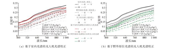
图7 室内光谱、野外原位光谱、无人机光谱和校正后的无人机光谱对比

Fig.7 Comparison of indoor spectrum, field in-situ spectrum, UAV spectrum and calibrated UAV spectrum

对校正后的无人机光谱进行MSC+FDR处理后,分别利用MLR,PLSR和RF建模,结果如图8所示。基于室内光谱的无人机光谱校正的3种模型精度均高于基于野外原位光谱的无人机光谱校正模型,说明用室内光谱作为参照光谱进行校正的效果最佳。此外,用室内光谱对无人机光谱进行校正后的3种模型建模集 $R_{c a l}^{2}$ 和验证集 $R_{v a l}^{2}$ 均大于0.88,而原始无人机光谱的建模集 $R_{c a l}^{2}$ 和验证集 $R_{v a l}^{2}$ 均小于0.88,说明校正后的无人机光谱能够提高模型精度。

图8

新窗口打开| 下载原图ZIP| 生成PPT

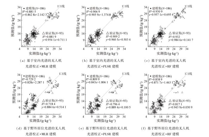
图8 校正后的无人机光谱数据的各模型预测值与实测值散点图

Fig.8 Scatter of measured value and predicted value from corrected UAV spectral data models

3.5 基于无人机高光谱最优估算模型的SOC含量制图

首先用实际采样点基于无人机高光谱最优估算模型(MSC+FDR)建立每个试验区SOC含量与特征波段的回归方程式,其次在ENVI软件的波段计算器中将回归方程式代入无人机高光谱图像中进行SOC制图,最终得到3个农田区SOC含量的分级制图结果,如图9所示。从图9中可以明显看出,A区的SOC含量主要为I级,B区的SOC含量主要为III级,C区的SOC含量主要为IV级。

图9

新窗口打开| 下载原图ZIP| 生成PPT

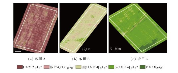
图9 SOC含量分级制图结果

Fig.9 Results of hierarchical mapping of soil organic carbon content

为了验证制图结果的准确性,将各农田区的采样点实测值与无人机影像的反演值进行对比,结果如图10所示。可以看出,3个农田区对应样点的预测值均能较好地拟合采样点的实测值,R²均在0.89以上,验证精度较高,满足制图要求。3个试验区的反演精度从高到低排序为: C区>B区>A区。

图10

新窗口打开| 下载原图ZIP| 生成PPT

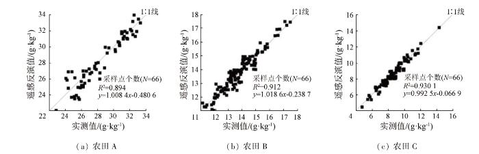
图10 各农田区采样点实测值与预测值对比结果

Fig.10 Results of comparison between measured values and predicted values in three farmland area

对3个农田区的SOC制图结果进行分级统计,得到各级别面积、占比和SOC含量情况,如表4所示。A区SOC含量均值为28.88 g·kg^-1,以I级为主,面积为16 532 m²,占比为82.66 %; 其次是II级,占比13.47 %,剩余等级面积占比均不到3 %,SOC含量整体空间分布均匀。B区SOC含量均值为13.52 g·kg^-1,以III级为主; 其次是II级和IV级,剩余等级面积占比均不超过1 %,在东南方向出现大量低值,而东北方向出现高值,SOC整体分布呈现出较强的空间差异性。C区SOC含量均值为8.54 g·kg^-1,以IV级为主,其次是V级和III级。各农田区平均SOC含量从高到低排序为: A区>B区>C区,这与实验室测定的SOC含量值较为一致。

表4 各农田区的有机碳含量及各等级面积的百分比

Tab.4 Organic carbon content in each farmland area

农田	等级Ⅰ		等级Ⅱ		等级Ⅲ		等级Ⅳ		等级Ⅴ		有机碳含量/(g·kg^-1)
农田	面积/m²	占比/%	面积/m²	占比/%	面积/m²	占比/%	面积/m²	占比/%	面积/m²	占比/%	均值	最小	最大
A区	16 532	82.66	2 694	13.47	576	2.88	128	0.64	70	0.35	28.88	5.18	33.66
B区	376	0.94	2 976	7.44	33 676	84.19	2 608	6.52	364	0.91	13.52	5.58	23.39
C区	265	0.79	312	0.93	2117	6.3	28 705	85.43	2 201	6.55	8.54	4.59	23.31

新窗口打开| 下载CSV

4 讨论

高光谱数据中常含噪声和冗余信息,对光谱数据进行预处理,能有效降低背景噪声的影响,增加光谱与SOC的相关性,优化特征波段筛选,提高建模精度^[25]。本文通过将无变换和7种变换方式的光谱与SOC含量做相关性分析发现,使用对数变换后的建模精度不佳,可能原因是对数变换在放大光谱特征波段的同时也增加了噪声和其他无关信息的干扰,同样在殷彩云等^[26]的研究中也发现对数变换对模型精度的提高不明显。经过MSC+FDR变换的相关系数最高,并且通过将MSC+FDR变换后的特征波段进行建模,其建模精度均高于其他变换方式,说明这种变换方式能够有效增强光谱特征,研究区SOC对MSC+FDR变换的光谱响应能力最好。SOC的高相关性可能是由于可见光—近红外波段中存在N-H和C-H的倍频峰和合频峰,能够让土壤中的碳元素在可见光—近红外波段范围内存在明显的响应波段。同时,这种变换在放大光谱特征波段的同时也能缩小噪声和无关因素的干扰^[27],这在一定程度上也会增加光谱相关性。此外,该变换中MSC能够有效增强光谱特征,SOC对这种变换的光谱响应能力较好,再加上FDR变化后更容易找到相关性高的波段,这与陈玮等^[28]的研究结果一致。本研究中的其他变换方法对模型精度有不同程度的提高,这一结果和张东辉等^[29]的研究相似。

将特征波段选入MLR,PLSR和RF这3种模型来预测SOC含量,其中MLR模型精度最低,这可能的原因是特征波段中存在的线性相关性不能完全消除,致使一部分重叠信息被反复利用^[30]。PLSR模型的精度优于前者,可能的原因是该模型能对光谱数据进行降维处理,能更有效地把握系统信息和噪声,有效保留关键的光谱信息^[31]。本文还选用了RF这种非线性模型进行SOC含量估算建模,发现RF模型较PLSR建模精度有大幅提高,这可能的原因是RF模型的稳定性更高、抗噪声能力更强、数据适应能力强且不容易发生过拟合现象^[32]。

肖艳等^[33]用室内光谱对黑龙江省的黑土有机质含量进行了估算,建模结果表明R²为0.91,具有较好的估算能力,这与本研究中的室内光谱建模结果较为一致; 纪文君^[27]采用野外原位测量的vis-NIR光谱对SOC含量进行了预测,建模精度R²为0.807,结果表明野外原位光谱可以对SOC进行定量预测,这与本研究结果一致; 杨晓宇等^[34]使用与本文相同的无人机高光谱(波段范围为400~1 000 nm)对松辽平原农田土壤有机质进行了估算,建模精度R²为0.73,这与本研究的无人机光谱建模精度相似。

罗德芳等^[35]的研究表明去除土壤水分能够有效提高建模精度,本研究的结果与此研究一致。这是因为光谱直接转换法能有效结合室内光谱和无人机光谱数据,通过室内光谱生成的转换矩阵对无人机光谱进行校正,获得“相对真值”,较好地保持无人机数据的信息特征^[36],最终用校正后的无人机数据去建模和制图,探讨无人机遥感在农田SOC反演中的有效性和适用性,把无人机影像真正用于农田管理并服务于农业生产。

无人机高光谱影像SOC含量制图结果表明,3个农田区SOC含量在空间上表现出较大的差异性。A区SOC含量最高,B区次之,C区最低,平均值分别为28.88 g·kg^-1 (A区)、13.52 g·kg^-1 (B区)与8.54 g·kg^-1 (C区)。具体而言,A区SOC整体空间分布均匀,82.66 %为等级I,低值较少,零星散落于区域南侧,但A区为收割后未进行翻耕土壤,有庄稼秸秆存在,导致反演精度最低。B区由于受翻地的影响,地表发生形变,导致SOC整体分布呈现出较强的空间差异性^[37],低值分布于区域东南部,高值位于B区中部。C区经过翻地后进行了冬灌,造成SOC从地表裂缝处流失,导致SOC含量的分布扰乱程度严重,占比最高的IV级达到C区面积的85.43 %,高值和低值的分化明显,整体SOC含量均值最低。本研究还存在一些不足,例如在A农田区中由于庄稼秸秆的存在而影响光谱曲线,从而导致制图精度最低,在今后的研究中应考虑对地表秸秆残留物的去除,以此提高建模精度。

5 结论

本研究立足于青海湟水流域内的3个典型农田区的所有土壤样品含量进行建模,SOC含量的取值范围为4.79~33.35 g·kg^-1。结果表明:

1)除对无人机光谱进行对数变换后的MLR模型不能估算有机碳外(RPD为1.375),3种光谱数据的原始光谱和所有转换方法都具有估算SOC的能力,其中实验室光谱的精度最高,野外原位光谱的精度次之,无人机光谱的精度最低。

2)SOC含量与MSC+FDR变换后的光谱反射率相关性最高,特征波段为429~449 nm, 498~527 nm, 830~861 nm和869 nm。

3)在3种建模结果中,MLR模型精度最低,PLSR模型精度次之,RF模型精度最高。

4)3个农田区的反演精度均满足制图要求,其中A农田区SOC含量均值最高,整体空间分布均匀; B农田区SOC整体分布呈现出较强的空间差异性; C农田区SOC含量均值最低,高值和低值的分化明显。

参考文献

原文顺序

文献年度倒序

文中引用次数倒序

被引期刊影响因子

[1]

Y W

, Duan

X W

, Li

et al.

Interactive effects of land use and soil erosion on soil organic carbon in the dry-hot valley region of southern China

[J]. Catena, 2021, 201(155):105187.