
1 引言
随着研究人员的深入挖掘,发现通过将光谱信息和空间信息有效融合,可大大改善高光谱遥感图像的分类结果。由于局部空间区域内有较大的概率属于同一类别,且其光谱值也可能非常相近。因此,一种基于分割的高光谱图像分类方法[6,7,8,9,10]被提出,这类方法通过提取像元间相邻的空间信息实现图像分割,且可取得较好的分类效果,但大部分算法时间复杂度较高。为解决这一问题,李旭超等[11]提出了马尔可夫随机场方法,该方法通过将像素空间关系紧密地结合在一起,可用低阶的马尔可夫随机场描述像素间的作用关系,减少方法时间复杂度。由于该方法对纹理结构要求高,分割效果也需进一步改进。在此基础上,Tarabalka等[12]提出了一种基于markers的最小传播森林分割分类方法(minimum spanning forest,MSF),充分考虑邻近像素的空间与光谱信息,通过选取粗分类中可信度最高的像素点为标记点(markers)作为MSF的初始点,实现对像素点区域的平滑与精准分割,取得了较好的实验效果。
以上结合空间与光谱信息的分类方法虽然取得了较好的效果,但性能上仍有进一步提升的空间。为此,本文提出一种融合递归滤波(recursive filtering,RF)与KNN(k-nearest neighbor)的高光谱遥感图像分类方法,利用RF算法有效去除高光谱图像中的噪声,强化空间结构,充分利用地物目标的空间上下文信息,然后利用KNN算法计算图像像素点的欧式距离,进行决策分类。
2 方法原理
2.1 RF算法
RF算法的原理为对给定的变换域
式中:
式中:
2.2 KNN算法
NN(nearest neighbor)分类器的原理是通过距离度量为测试样本找到最邻近的训练样本,根据训练样本类别来决策测试样本的类别。KNN算法基于此原理,已知训练样本标签的类别,寻找测试样本的
式中:
2.3 RF-KNN分类方法
本文提出的RF-KNN分类方法实现过程主要为4步骤: ①利用主成分分析法(principal component analysis,PCA)对高光谱图像进行降维; ②对降维后的PCA分量图像进行RF,强化空间结构信息; ③计算测试样本与每一类训练样本的欧式距离; ④选取与测试样本距离最近的k个测试样本,根据k个训练样本的类别判断测试样本所属类别。
2.4 评价指标
在完成高光谱图像分类后,需要对高光谱图像的分类结果进行客观评价。通常依据地面参考数据,评估分类结果的准确性。采用4个常见的高光谱图像分类精度指标来衡量分类算法的精度: 每类分类精度(class accuracy,CA)、整体分类精度(overall accuracy,OA)、平均分类精度(average accuracy,AA)以及Kappa系数。同时,为了避免实验存在随机误差,每个实验重复20次记录平均结果与方差。
3 实验数据及参数分析
3.1 实验数据集
采用Indian Pines和 Salinas这2个高光谱数据集作为实验数据集,分别如图1和图2所示。2景遥感图像均来自AVIRIS(airborne visible infra-red imaging spectrometer)光谱仪收集到的高光谱遥感图像,Indian Pines影像为1992年在印第安纳州西北部地区影像,具有20 m的空间分辨率,由于噪声和水吸收等因素除去其中的20个波段,剩余200个波段,图像范围大小为145像素×145像素,其中包含16种地物。Salinas影像为美国加利福尼亚州萨利纳斯山谷地区影像,含224个波段,空间分辨率为3.7 m,图像范围大小为512像素×217像素,其中包含16种地物,由于噪声和水吸收等因素亦除去遥感图像中的20个波段。
图1
图2
3.2 实验参数分析
为了得到最佳的分类精度,对RF算法中的
通过确定RF算法中
图3
图3
RF参数对不同数据集分类精度的影响分析
Fig.3
Analysis of RF parameters on classification accuracy in different data sets
在分析
分析最邻近数k对分类精度的影响时,仅改变k参数,其余参数选为常数。如图4所示,当k=1时,2个数据集都能获得最高的分类精度,分别为98.96%和99.51%。随着k的增加,引入的噪声数据也会相应增加,导致分类精度下降。
图4
图4
最近邻数k对不同数据集分类精度的影响分析
Fig.4
Analysis of the number of nearest neighbor on classification accuracy in different data sets
此外,特征维度Dim也是影响高光谱分类精度的重要因素。实验分析如图5所示。
图5

图5
维度对不同数据集分类精度的影响分析
Fig.5
Analysis of dimension on classification accuracy in different data sets
当Dim=4时,分类精度较低。其原因是图像降维过程中会丢失大量有用的光谱信息,使分类精度降低。随着Dim增加,2个数据集的分类精度变化趋势类似,都是先增加再保持不变。在Indian Pines数据集上,当Dim=20时,分类精度最高; 在Salinas数据集上,当Dim=30时,分类精度最高。
4 实验结果与分析
4.1 不同分类算法比较
为了验证本文提出方法的优越性,实验比较了本文提出的方法与传统的分类算法和几种空谱分类算法的分类效果,其算法包括: 传统分类算法SVM[5]、稀疏表示分类(sparse representation classification,SRC)[20]算法、联合稀疏表示分类算法(joint sparse representation classification,JSRC)[21]、扩展形态特征(extended morphological profiles,EMP)算法[22]、边缘保持滤波(edge preserving filtering,EPF)的算法[23]、基于图像融合和递归滤波(image fusion and recursive filtering,IFRF)的算法[19]以及逻辑回归与多层回归(logistic regression and multi-level logistic,LMLL)算法[24]。在进行实验比较之前,先设置不同类算法的参数。SVM的最佳参数通过10次交叉验证确定。对于EMP算法,利用HSI的前3个主成分分量,形态学算子的尺寸依次递增2个像素,共进行4次形态学开闭和重构运算,构建多尺度形态学特征。对于EPF算法,使用前4个主要部件,圆形结构元件、二阶梯形增量及4个开口和关闭构造形态轮廓进行参数设置。对于SRC,JSRC,IFRF和LMLL算法,实验均采用默认参数,通过Matlab编写代码实现。
4.2 实验结果
4.2.1 Indian Pines数据集
图6
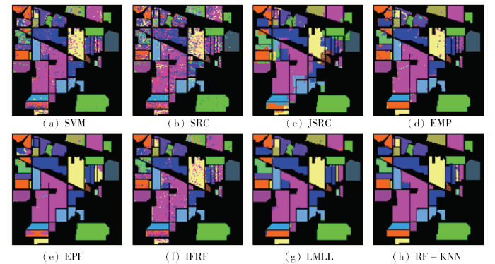
图6
不同算法在Indian Pines数据集的分类结果(10%训练样本)
Fig.6
Classification results of different algorithms in the Indian Pines data set (10% of training samples)
图7
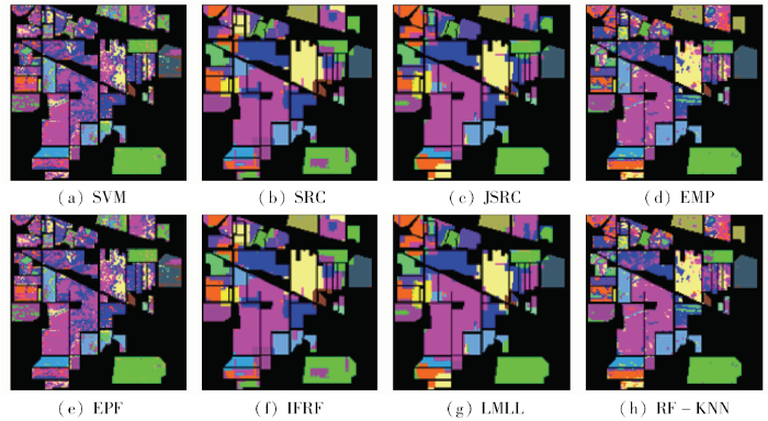
图7
不同算法在Indian Pines数据集的分类结果(1%训练样本)
Fig.7
Classification results of different algorithms in the Indian Pines data set (1% of training samples)
对于仅使用光谱信息的SVM分类算法而言,分类结果中噪声点较多,并且每种地物类型与实际地物类型对应关系错误率也较高,分类精度较低。相比SVM分类算法,EMP算法在分类时通过利用图像空间结构信息总是能获得更高的分类精度,然而在分类结果中一些“噪声”状的误分类仍然可见。相比EMP算法,EPF算法通过边缘保持滤波联合空间信息与光谱分类结果,能提升分类精度。对于本文提出的RF-KNN方法而言,不但利用RF算法平滑了噪声,增强空间结构,而且还结合空间邻域信息进行分类,分类精度优于其他空谱分类算法。当训练样本极少时,本文提出的方法依然能获得较好的分类精度。比如能准确地识别位于实验区右上方的地物类别。该方法通过有效地联合空间信息,对大多数地物类别的识别精度均优于其他空谱分类算法。
表1 Indian Pines高光谱图像不同算法分类精度(10%训练样本)
Tab.1
| 指标 类别 | 训练样 本/个 | 测试样 本/个 | SVM | SRC | JSRC | EMP | EPF | IFRF | LMLL | RF-KNN | |
|---|---|---|---|---|---|---|---|---|---|---|---|
| CA | Alfalfa | 10 | 36 | 79.31 (7.32) | 61.58 (10.62) | 94.44 (8.10) | 94.44 (2.78) | 97.86 (6.68) | 99.73 (0.85) | 94.44 (0.00) | 94.44 (0.00) |
| Corn-N | 143 | 1 285 | 78.49 (0.83) | 53.06 (2.96) | 93.81 (2.00) | 87.77 (2.06) | 95.95 (2.28) | 97.55 (0.99) | 94.75 (0.37) | 98.49 (0.56) | |
| Corn-M | 83 | 747 | 80.74 (2.78) | 50.33 (3.65) | 91.51 (1.19) | 92.74 (2.28) | 96.00 (2.56) | 98.59 (0.91) | 73.76 (0.00) | 98.69 (0.48) | |
| Corn | 34 | 203 | 67.72 (5.46) | 37.56 (3.80) | 91.74 (3.54) | 85.73 (5.36) | 92.21 (5.33) | 97.62 (1.29) | 98.59 (0.00) | 99.70 (0.44) | |
| Grass-M | 48 | 435 | 90.28 (2.20) | 83.77 (1.80) | 92.37 (3.38) | 92.00 (2.81) | 99.00 (0.88) | 98.96 (1.07) | 95.86 (0.00) | 97.33 (3.34) | |
| Grass-T | 23 | 707 | 89.28 (2.00) | 91.39 (1.22) | 93.55 (1.00) | 97.63 (0.67) | 95.15 (2.97) | 99.05 (0.63) | 100.00 (0.00) | 96.94 (1.83) | |
| Grass-P | 15 | 13 | 83.04 (13.35) | 82.00 (8.37) | 100.00 (0.00) | 94.44 (5.56) | 97.24 (6.40) | 91.43 (18.07) | 100.00 (0.00) | 100.00 (0.00) | |
| Hay-W | 28 | 450 | 97.47 (0.90) | 93.30 (0.92) | 99.02 (0.71) | 99.91 (0.13) | 99.99 (0.05) | 100.00 (0.00) | 100.00 (0.00) | 100.00 (0.00) | |
| Oats | 15 | 5 | 46.35 (9.95) | 55.00 (13.94) | 62.00 (40.25) | 100.00 (0.00) | 100.00 (0.00) | 81.82 (17.64) | 100.00 (0.00) | 100.00 (0.00) | |
| Soybean-N | 150 | 822 | 80.02 (2.17) | 66.17 (3.90) | 91.08 (1.93) | 88.88 (0.78) | 92.21 (4.48) | 96.84 (1.35) | 90.83 (0.00) | 99.12 (0.89) | |
| Soybean-M | 246 | 2 209 | 80.84 (2.11) | 70.16 (1.47) | 97.08 (1.16) | 95.38 (0.88) | 91.71 (4.46) | 98.07 (1.04) | 91.67 (0.00) | 99.29 (0.37) | |
| Soybean-C | 60 | 533 | 78.99 (3.24) | 45.51 (2.62) | 84.54 (4.64) | 86.83 (2.37) | 94.73 (3.60) | 98.08 (1.07) | 93.21 (0.34) | 98.16 (0.98) | |
| Wheat | 21 | 184 | 93.80 (2.63) | 91.74 (3.06) | 86.20 (2.89) | 99.24 (0.62) | 100.00 (0.00) | 97.60 (2.30) | 99.46 (0.00) | 99.02 (0.81) | |
| Woods | 127 | 1 138 | 91.96 (1.49) | 89.19 (1.51) | 99.51 (0.26) | 99.63 (0.26) | 95.11 (2.86) | 99.70 (0.35) | 97.98 (0.00) | 99.72 (0.40) | |
| Buildings | 35 | 351 | 73.95 (4.28) | 35.45 (1.85) | 92.08 (4.33) | 97.32 (1.69) | 95.27 (2.64) | 97.38 (1.69) | 94.87 (0.00) | 98.46 (1.47) | |
| Stone | 37 | 56 | 93.97 (4.13) | 89.88 (2.64) | 94.29 (4.96) | 98.57 (0.80) | 96.40 (3.11) | 95.98 (5.05) | 94.64 (0.00) | 99.64 (0.80) | |
| OA | — | — | 83.33 (0.77) | 68.47 (0.59) | 94.19 (0.57) | 94.41 (0.84) | 94.47 (1.80) | 98.23 (0.18) | 94.45 (0.78) | 98.82 (0.29) | |
| AA | — | — | 81.64 (1.30) | 68.51 (1.89) | 91.45 (1.27) | 94.41 (0.84) | 96.18 (0.89) | 96.79 (1.80) | 95.69 (0.51) | 98.65 (0.33) | |
| Kappa | — | — | 80.90 (0.90) | 64.02 (0.63) | 93.37 (0.65) | 92.77 (0.49) | 93.67 (2.07) | 97.98 (0.21) | 93.65 (0.90) | 98.69 (0.29) | |
表2 Indian Pines高光谱图像不同算法分类精度(1%训练样本)
Tab.2
| 指标 类别 | 训练样 本/个 | 测试样 本/个 | SVM | SRC | JSRC | EMP | EPF | IFRF | LMLL | RF-KNN | |
|---|---|---|---|---|---|---|---|---|---|---|---|
| CA | Alfalfa | 3 | 43 | 72.25 (5.43) | 63.26 (18.20) | 92.56 (9.21) | 87.44 (6.41) | 72.42 (30.15) | 88.35 (31.74) | 95.35 (0.00) | 95.35 (0.00) |
| Corn-N | 14 | 1 414 | 47.63 (7.37) | 40.07 (5.91) | 69.99 (6.50) | 57.39 (4.59) | 61.20 (8.91) | 83.17 (8.34) | 69.12 (0.42) | 83.97 (10.41) | |
| Corn-M | 8 | 822 | 55.60 (15.51) | 31.33 (6.92) | 55.28 (8.60) | 63.64 (7.29) | 73.96 (18.37) | 71.08 (10.79) | 44.09 (0.11) | 74.67 (14.06) | |
| Corn | 3 | 234 | 35.98 (11.21) | 25.37 (8.55) | 45.04 (15.61) | 29.79 (9.89) | 59.62 (33.29) | 70.28 (12.62) | 33.42 (0.19) | 92.22 (8.31) | |
| Grass-M | 6 | 477 | 74.25 (12.10) | 63.59 (10.07) | 70.23 (26.81) | 77.04 (9.38) | 90.54 (12.56) | 85.61 (9.82) | 69.18 (0.00) | 89.48 (3.16) | |
| Grass-T | 7 | 723 | 76.13 (6.57) | 77.25 (8.63) | 85.48 (3.41) | 86.07 (13.92) | 74.85 (6.53) | 90.66 (5.52) | 98.76 (0.00) | 97.10 (1.64) | |
| Grass-P | 3 | 25 | 30.57 (15.22) | 89.04 (5.76) | 92.00 (12.33) | 90.80 (9.25) | 81.41 (30.42) | 52.28 (25.97) | 96.00 (0.00) | 100.00 (0.00) | |
| Hay-W | 5 | 473 | 93.09 (5.37) | 73.82 (12.02) | 84.90 (8.79) | 94.82 (3.02) | 98.42 (2.99) | 100.00 (0.00) | 99.79 (0.00) | 100.00 (0.00) | |
| Oats | 3 | 17 | 18.99 (9.95) | 68.35 (20.16) | 94.12 (10.19) | 96.47 (7.44) | 48.01 (37.62) | 27.79 (20.58) | 100.00 (0.00) | 96.47 (7.89) | |
| Soybean-N | 10 | 962 | 53.88 (7.46) | 49.04 (8.64) | 71.10 (5.46) | 69.27 (9.05) | 70.51 (15.60) | 72.87 (10.46) | 73.80 (2.79) | 84.30 (4.51) | |
| Soybean-M | 24 | 2 431 | 59.35 (4.18) | 61.04 (4.71) | 82.59 (5.06) | 77.10 (6.22) | 66.08 (9.18) | 85.91 (4.45) | 79.66 (0.13) | 93.58 (4.15) | |
| Soybean-C | 6 | 587 | 38.95 (8.03) | 21.85 (6.44) | 48.07 (8.57) | 39.93 (7.11) | 56.11 (22.14) | 70.91 (12.35) | 55.54 (0.76) | 80.20 (9.34) | |
| Wheat | 2 | 203 | 84.36 (4.03) | 77.38 (11.01) | 79.61 (12.27) | 95.81 (1.89) | 96.16 (3.87) | 80.46 (12.73) | 99.31 (0.44) | 96.75 (2.38) | |
| Woods | 13 | 1 252 | 84.44 (2.87) | 80.95 (6.80) | 92.54 (7.27) | 87.61 (5.30) | 87.10 (5.07) | 92.88 (1.76) | 97.78 (0.04) | 92,99 (6.50) | |
| Buildings | 4 | 382 | 42.01 (10.72) | 19.04 (5.30) | 36.70 (7.27) | 61.52 (13.30) | 67.86 (24.93) | 80.08 (9.07) | 20.37 (0.79) | 83.66 (6.88) | |
| Stone | 3 | 90 | 96.89 (5.87) | 87.00 (4.84) | 96.89 (2.41) | 71.44 (25.08) | 93.81 (20.70) | 97.97 (10.17) | 74.89 (1.49) | 98.67 (0.93) | |
| OA | — | — | 60.60 (2.00) | 54.87 (1.63) | 74.04 (1.37) | 71.88 (2.25) | 71.00 (2.97) | 81.84 (2.88) | 86.72 (5.32) | 89.07 (1.17) | |
| AA | — | — | 57.46 (2.63) | 58.02 (2.14) | 74.82 (2.74) | 74.13 (3.18) | 74.88 (5.28) | 78.14 (3.00) | 84.91 (4.79) | 87.57 (1.32) | |
| Kappa | — | — | 54.59 (2.16) | 48.47 (1.86) | 70.12 (1.52) | 67.88 (2.52) | 66.24 (3.70) | 79.29 (3.28) | 84.77 (6.11) | 91.21 (0.84) | |
由表1和表2可知,本文提出的RF-KNN方法在OA,AA和Kappa指标上有相对的优势。SRC的分类算法精度最低,SVM算法在训练样本占地面参考数据10%的情况下,能够有效地区分Wheat,Woods和Stone等光谱区分度较大的地物,然而由于未考虑高光谱图像的空间信息,对于一些光谱类似的地物,分类识别精度不高。例如,Oats的分类精度仅为46.35%。相比SVM算法,其他空谱分类算法能提升分类精度,但对某些类别的分类精度较低,比如对于Soybean的识别。本文的RF-KNN方法能取得最高的分类精度。例如Grass-P,Hay-W和Oats的分类精度能达到100%,大多数类别上的分类精度均高于98%; 相比SRC算法,对于Alfalfa的识别,提高了32.86%。在训练样本占地面参考数据1%的情况下,大部分算法识别精度明显下降,而本文方法依然能获得最佳的分类精度,且对Grass-P和Hay-W的分类精度仍保持为100%。
4.2.2 Salinas数据集
在Salinas数据集中,将所有数据分为训练样本和测试样本。随机选取参考数据中的2%作为训练样本,其余作为测试样本。并进一步改变训练样本的数量进行实验,随机选取参考数据中的0.2%作为训练样本,剩下99.8%的参考数据作为测试样本。Salinas数据集不同算法分类结果如图8和图9所示,SVM算法分类结果中噪声点较多。与仅使用光谱信息的SVM算法相比,JSRC算法通过联合空间信息能有效去除这种类似噪声的误分类,提高了分类精度。相比其他7种高光谱遥感图像分类算法,本文所提出的RF-KNN方法总能获得更高的分类精度,其原因在于利用RF算法有效地平滑了噪声,强化了地物轮廓,对图像区域边缘划分效果较好。随着训练样本数量的减少,JSRC,EPF和LMLL算法分类结果中出现明显误分类现象,IFRF算法和RF-KNN方法均能在训练样本减少时较好地区分各种地物覆盖类别。虽然两者均有去除图像噪声与增强影像空间结构的特性,但是相比于IFRF算法,RF-KNN方法通过加入空间近邻信息进一步提高了分类精度。分类精度分别如表3和表4所示。
图8
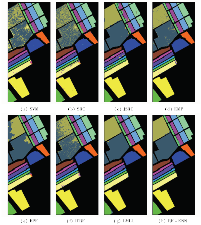
图8
不同算法在Salinas数据集的分类结果(2%训练样本)
Fig.8
Classification results of different algorithms in the Salinas data set (2% of training samples)
图9

图9
不同算法在Salinas数据集的分类结果(0.2%训练样本)
Fig. 9
Classification results of different algorithms in the Salinas data set (0.2% of training samples)
表3 Salinas高光谱图像不同算法分类精度(2%训练样本)
Tab.3
| 指标 类别 | 训练样 本/个 | 测试样 本/个 | SVM | SRC | JSRC | EMP | EPF | IFRF | LMLL | RF-KNN | |
|---|---|---|---|---|---|---|---|---|---|---|---|
| CA | Weeds_1 | 40 | 1 969 | 100.00 (0.00) | 98.36 (0.65) | 100.00 (0.00) | 99.80 (0.00) | 100.00 (0.00) | 100.00 (0.00) | 100.00 (0.00) | 100.00 (0.00) |
| Weeds_2 | 73 | 3 653 | 97.19 (0.53) | 98.52 (0.45) | 99.41 (0.67) | 99.56 (0.34) | 100.00 (0.00) | 99.99 (0.02) | 100.00 (0.00) | 99.86 (0.13) | |
| Fallow | 38 | 1 938 | 94.60 (1.45) | 96.76 (1.21) | 99.16 (0.77) | 99.54 (0.27) | 94.84 (1.61) | 99.88 (0.08) | 99.69 (0.15) | 100.00 (0.00) | |
| Fallow_P | 26 | 1 368 | 97.63 (1.11) | 99.26 (0.33) | 88.67 (5.45) | 98.30 (1.20) | 98.02 (0.56) | 97.84 (0.92) | 98.26 (2.88) | 97.35 (2.34) | |
| Fallow_S | 52 | 2 626 | 98.55 (0.54) | 94.39 (0.68) | 84.03 (2.06) | 96.77 (0.46) | 99.94 (0.05) | 99.47 (0.98) | 99.06 (0.28) | 98.64 (0.89) | |
| Stubble | 79 | 3 880 | 99.97 (0.05) | 99.69 (0.10) | 98.20 (1.33) | 99.60 (0.38) | 99.98 (0.02) | 100.00 (0.00) | 100.00 (0.00) | 99.76 (0.18) | |
| Celery | 70 | 3 509 | 99.40 (0.31) | 99.27 (0.14) | 95.10 (2.08) | 99.58 (0.09) | 99.84 (0.17) | 99.81 (0.11) | 99.94 (0.00) | 99.93 (0.05) | |
| Graps | 225 | 11 046 | 74.60 (1.74) | 73.62 (1.49) | 98.47 (0.23) | 96.38 (0.91) | 84.10 (4.04) | 99.64 (0.14) | 92.72 (0.06) | 99.87 (0.19) | |
| Soil | 124 | 6 079 | 99.62 (0.03) | 97.89 (0.93) | 99.99 (0.01) | 99.84 (0.23) | 99.18 (0.32) | 99.92 (0.12) | 100.00 (0.00) | 100.00 (0.00) | |
| Corn | 21 | 3 257 | 79.07 (5.21) | 78.13 (3.72) | 89.60 (3.36) | 93.38 (1.17) | 99.21 (0.83) | 99.64 (0.42) | 89.72 (1.99) | 98.66 (0.73) | |
| Lettuce_4wk | 21 | 1 047 | 86.93 (4.99) | 96.58 (2.71) | 88.83 (4.86) | 96.85 (1.53) | 96.97 (1.27) | 99.20 (0.30) | 95.52 (0.77) | 97.06 (2.52) | |
| Lettuce_5wk | 38 | 1 889 | 97.96 (0.49) | 99.72 (0.58) | 94.55 (0.99) | 99.52 (0.98) | 99.46 (0.63) | 98.82 (1.22) | 100.00 (0.00) | 99.68 (0.40) | |
| Lettuce_6wk | 18 | 898 | 98.47 (0.85) | 97.34 (0.43) | 83.78 (5.46) | 98.57 (1.17) | 98.58 (1.62) | 99.01 (1.22) | 97.16 (0.13) | 91.76 (8.28) | |
| Lettuce_7wk | 20 | 1 050 | 86.93 (4.81) | 92.69 (2.17) | 79.62 (5.57) | 96.13 (1.75) | 98.71 (0.53) | 98.16 (1.25) | 97.52 (0.04) | 98.84 (0.66) | |
| Vinyard_U | 140 | 7 128 | 66.51 (5.39) | 61.41 (1.96) | 97.39 (0.47) | 94.23 (1.16) | 91.82 (2.37) | 99.88 (0.16) | 68.43 (1.31) | 99.01 (0.44) | |
| Vinyard_T | 36 | 1 771 | 96.88 (2.12) | 95.57 (2.75) | 99.64 (0.18) | 99.31 (0.39) | 99.75 (0.44) | 99.97 (0.05) | 97.33 (0.48) | 100.00 (0.00) | |
| OA | — | — | 87.57 (1.08) | 86.69 (0.54) | 95.98 (0.53) | 97.53 (0.20) | 94.78 (1.23) | 99.42 (0.10) | 93.23 (0.19) | 99.46 (0.12) | |
| AA | — | — | 92.14 (0.85) | 92.45 (0.54) | 93.53 (1.09) | 97.96 (0.25) | 97.53 (0.32) | 99.15 (0.10) | 95.95 (0.21) | 99.29 (0.14) | |
| Kappa | — | — | 86.14 (1.19) | 85.17 (0.61) | 95.53 (0.59) | 97.25 (0.22) | 94.17 (1.38) | 99.62 (0.11) | 92.44 (0.21) | 98.78 (0.54) | |
表4 Salinas高光谱图像不同算法分类精度(0.2%训练样本)
Tab.4
| 指标 类别 | 训练样 本/个 | 测试样 本/个 | SVM | SRC | JSRC | EMP | EPF | IFRF | LMLL | RF-KNN | |
|---|---|---|---|---|---|---|---|---|---|---|---|
| CA | Weeds_1 | 4 | 2 005 | 99.97 (0.04) | 96.22 (1.21) | 100.00 (0.00) | 95.22 (9.57) | 100.00 (0.00) | 95.83 (5.08) | 99.56 (0.41) | 94.54 (8.02) |
| Weeds_2 | 8 | 3 718 | 94.87 (5.09) | 97.60 (1.88) | 99.70 (0.32) | 98.95 (0.47) | 99.96 (0.08) | 99.77 (0.49) | 99.74 (0.13) | 99.09 (3.72) | |
| Fallow | 4 | 1 972 | 86.58 (4.53) | 81.85 (13.07) | 92.11 (9.31) | 75.79 (17.54) | 88.15 (1.26) | 98.00 (2.63) | 99.62 (0.18) | 100.00 (0.00) | |
| Fallow_P | 3 | 1 391 | 97.17 (0.48) | 99.07 (0.49) | 56.96 (18.30) | 99.01 (0.53) | 97.47 (0.62) | 91.10 (8.78) | 56.70 (2.61) | 76.62 (8.58) | |
| Fallow_S | 5 | 2 673 | 97.94 (0.80) | 90.47 (4.61) | 79.07 (6.65) | 94.52 (2.44) | 93.95 (7.58) | 98.54 (2.22) | 99.13 (0.38) | 93.52 (4.98) | |
| Stubble | 8 | 3 951 | 99.98 (0.06) | 99.59 (0.10) | 99.83 (0.14) | 97.05 (2.45) | 99.97 (0.04) | 100.00 (0.00) | 99.52 (0.21) | 97.77 (1.28) | |
| Celery | 7 | 3 572 | 95.19 (3.65) | 98.55 (1.62) | 96.41 (1.60) | 99.34 (0.21) | 97.79 (3.06) | 99.39 (0.69) | 99.73 (0.09) | 98.64 (1.49) | |
| Graps | 21 | 11 250 | 64.31 (4.69) | 69.24 (5.61) | 89.36 (2.82) | 85.68 (7.31) | 70.03 (7.78) | 95.22 (5.66) | 88.20 (1.35) | 93.77 (4.58) | |
| Soil | 11 | 6 192 | 99.59 (0.03) | 96.97 (0.59) | 99.61 (0.67) | 99.26 (0.64) | 92.56 (10.95) | 98.58 (3.35) | 99.01 (1.16) | 100.00 (0.00) | |
| Corn | 3 | 3 275 | 77.73 (8.42) | 54.75 (20.40) | 79.57 (1.88) | 73.97 (16.68) | 91.63 (4.47) | 98.94 (0.70) | 90.02 (3.62) | 97.92 (1.69) | |
| Lettuce_4wk | 3 | 1 065 | 64.29 (6.73) | 93.12 (3.49) | 80.56 (9.38) | 94.80 (1.60) | 76.28 (28.19) | 98.75 (0.40) | 92.94 (0.75) | 88.26 (5.87) | |
| Lettuce_5wk | 4 | 1 923 | 92.36 (3.56) | 97.32 (3.13) | 71.45 (13.17) | 99.95 (0.12) | 96.28 (6.13) | 92.19 (3.75) | 100.00 (0.00) | 80.09 (14.87) | |
| Lettuce_6wk | 2 | 914 | 89.61 (10.32) | 97.19 (1.66) | 56.09 (13.08) | 98.49 (0.44) | 86.04 (8.46) | 83.58 (16.15) | 97.55 (0.65) | 71.66 (19.57) | |
| Lettuce_7wk | 2 | 1 068 | 71.56 (18.02) | 81.08 (4.11) | 94.41 (1.47) | 92.57 (3.86) | 98.83 (0.77) | 81.37 (17.11) | 96.66 (1.97) | 60.28 (22.83) | |
| Vinyard_U | 13 | 7 255 | 45.34 (4.69) | 53.50 (6.93) | 70.38 (8.04) | 72.99 (8.62) | 87.61 (10.47) | 89.90 (6.73) | 72.37 (2.60) | 96.61 (1.49) | |
| Vinyard_T | 4 | 1 803 | 93.56 (10.78) | 73.55 (11.52) | 96.14 (4.08) | 86.88 (8.76) | 99.93 (0.09) | 99.63 (1.17) | 96.04 (5.00) | 99.80 (0.45) | |
| OA | — | — | 79.33 (1.99) | 81.14 (1.39) | 87.44 (1.02) | 89.32 (2.00) | 86.23 (2.51) | 94.40 (2.08) | 91.48 (0.87) | 94.93 (1.26) | |
| AA | — | — | 85.63 (1.86) | 86.25 (1.21) | 85.10 (0.88) | 91.53 (1.38) | 92.28 (1.89) | 94.05 (1.98) | 92.93 (0.91) | 94.69 (1.40) | |
| Kappa | — | — | 77.14 (2.15) | 78.97 (1.52) | 85.99 (1.14) | 88.08 (2.22) | 84.55 (2.88) | 94.18 (2.32) | 90.50 (0.97) | 94.41 (3.05) | |
5 结论
在本文所提出的基于递归滤波和KNN的高光谱图像分类方法较好地结合光谱和空间邻域信息,有效降低了错误分类概率。该方法通过在2个经典实验数据库上进行实验并且与其他算法进行了对比验证,结果表明,与现有高光谱遥感图像分类算法相比,该方法在不同训练样本下都具有较好的分类性能,并且具有较好的鲁棒性,为高光谱遥感图像分类领域提供了新的研究思路与方法。但在实验过程中,该方法的时间复杂度较高,因此如何有效降低该方法的时间复杂度是下一步研究的重点。
志谢: 康旭东博士提供了EPF和IFRF算法代码,李军教授提供了LMLL算法代码,在此一并表示感谢。最后,感谢李树涛教授和康旭东博士对论文给出的深刻意见。
参考文献
航天高光谱成像技术研究现状及展望
[J].
DOI:10.3788/LOP50.010008
URL
[本文引用: 1]

自1997年8月23日首颗高光谱卫星LEWIS发射以来,航天高光谱成像技术走过了15年的路程,我国在该领域的技术也取得了跨越式的发展。当前我国正按照国家中长期科技规划,努力构建下一代高分辨率对地观测系统,深入全面地总结过去若干年的航天高光谱成像技术发展情况,并分析发达国家的发展计划,对制定我国的航天高光谱成像技术发展战略具有重要意义。从当前的主流高光谱分光技术、应用情况和发展趋势三个方面进行了全面的分析总结,认为民用高光谱成像系统应该朝着宽幅、定量化和应用细分的方向发展;军用高光谱成像系统的发展重点应该是高空间分辨率、宽波段以及快速信息处理技术。
Status and prospect of space-borne hyperspectral imaging technology
[J].
Detection algorithms for hyperspectral imaging applications
[J].
DOI:10.1109/79.974724
URL
[本文引用: 1]
We introduce key concepts and issues including the effects of atmospheric propagation upon the data, spectral variability, mixed pixels, and the distinction between classification and detection algorithms. Detection algorithms for full pixel targets are developed using the likelihood ratio approach. Subpixel target detection, which is more challenging due to background interference, is pursued using both statistical and subspace models for the description of spectral variability. Finally, we provide some results which illustrate the performance of some detection algorithms using real hyperspectral imaging (HSI) data. Furthermore, we illustrate the potential deviation of HSI data from normality and point to some distributions that may serve in the development of algorithms with better or more robust performance. We therefore focus on detection algorithms that assume multivariate normal distribution models for HSI data
Hyperspectral remote sensing data analysis and future challenges
[J].
DOI:10.1109/MGRS.2013.2244672
URL
[本文引用: 1]
Hyperspectral remote sensing technology has advanced significantly in the past two decades. Current sensors onboard airborne and spaceborne platforms cover large areas of the Earth surface with unprecedented spectral, spatial, and temporal resolutions. These characteristics enable a myriad of applications requiring fine identification of materials or estimation of physical parameters. Very often, these applications rely on sophisticated and complex data analysis methods. The sources of difficulties are, namely, the high dimensionality and size of the hyperspectral data, the spectral mixing (linear and nonlinear), and the degradation mechanisms associated to the measurement process such as noise and atmospheric effects. This paper presents a tutorial/overview cross section of some relevant hyperspectral data analysis methods and algorithms, organized in six main topics: data fusion, unmixing, classification, target detection, physical parameter retrieval, and fast computing. In all topics, we describe the state-of-the-art, provide illustrative examples, and point to future challenges and research directions.
高光谱遥感图像最大似然分类问题及解决方法
[J].
DOI:10.3969/j.issn.1672-3767.2005.03.017
URL
[本文引用: 1]
利用最大似然分类器对高光谱遥感图像分类时,由于波段数目多、波段间的相关度大,使协方差矩阵的行列式近似于奇异,因而导致了不合理的分类结果。本文调整了波段协方差矩阵对分类的影响,改进了最大似然分类判决函数,利用改进后的判决函数进行分类,试验证明这种方法是有效的。另外,根据图像特征和经验对图像进行波段选择,也是改善高光谱遥感分类效果的有效途径。
The MLC’s problem in classification of hyperspectral RS image and its solving method
[J].
Classification of hyperspectral remote sensing images with support vector machines
[J].
DOI:10.1109/TGRS.2004.831865
URL
[本文引用: 2]
This paper addresses the problem of the classification of hyperspectral remote sensing images by support vector machines (SVMs). First, we propose a theoretical discussion and experimental analysis aimed at understanding and assessing the potentialit...
Advances in spectral-spatial classification of hyperspectral images
[J].
DOI:10.1109/JPROC.2012.2197589
URL
[本文引用: 1]
Recent advances in spectral-spatial classification of hyperspectral images are presented in this paper. Several techniques are investigated for combining both spatial and spectral information. Spatial information is extracted at the object (set of pixels) level rather than at the conventional pixel level. Mathematical morphology is first used to derive the morphological profile of the image, which includes characteristics about the size, orientation, and contrast of the spatial structures present in the image. Then, the morphological neighborhood is defined and used to derive additional features for classification. Classification is performed with support vector machines (SVMs) using the available spectral information and the extracted spatial information. Spatial postprocessing is next investigated to build more homogeneous and spatially consistent thematic maps. To that end, three presegmentation techniques are applied to define regions that are used to regularize the preliminary pixel-wise thematic map. Finally, a multiple-classifier (MC) system is defined to produce relevant markers that are exploited to segment the hyperspectral image with the minimum spanning forest algorithm. Experimental results conducted on three real hyperspectral images with different spatial and spectral resolutions and corresponding to various contexts are presented. They highlight the importance of spectral-spatial strategies for the accurate classification of hyperspectral images and validate the proposed methods.
超像素分割算法研究综述
[J].
DOI:10.3969/j.issn.1001-3695.2014.01.002
URL
[本文引用: 1]
超像素能够捕获图像冗余信息,降低后续处理任务复杂度,已受到了国内外研究者的日益关注。首先分析了超像素分割领域的发展现状,以基于图论的方法和基于梯度下降的方法为视角,对现有超像素分割方法进行归纳和论述。在此基础上,就目前常用的超像素分割算法进行了实验对比,分析各自的优势和不足。最后,对超像素分割技术的最新应用进行了介绍和展望。
Review on superpixel segmentation algorithms
[J].
基于多层分割的面向对象遥感影像分类方法研究
[J].<p>利用ALOS数据,在Definiens Developer 7软件中用分形网络演化法(FNEA)进行多级分割,获取影像对象。综合运用对象的光谱、空间特征和不同层对象之间的关系,提取了湖北省洪湖市试验区土地覆盖与土地利用信息。最后,用一种基于单层分割的面向对象分类方法和基于像素的最大似然法与这种基于多级分割的面向对象分类方法进行了对比分析。结果表明,基于多级分割的面向对象分类方法,不仅克服了基于像素的最大似然法出现的“椒盐”现象,在分类精度上较这两种分类方法也有大幅度的提高。</p>
Study on object-oriented remote sensing image classification based on multi-levels segmentation
[J].
Watersheds in digital spaces:An efficient algorithm based on immersion simulations
[J].
DOI:10.1109/34.87344
URL
[本文引用: 1]
Summary: A fast and flexible algorithm for computing watersheds in digital gray-scale images is introduced. A review of watersheds and related motion is first presented, and the major methods to determine watersheds are discussed. The algorithm is based on an immersion process analogy, in which the flooding of the water in the picture is efficiently simulated using of queue of pixel. It is described in detail provided in a pseudo C language. The accuracy of this algorithm is proven to be superior to that of the existing implementations, and it is shown that its adaptation to any kind of digital grid and its generalization to n-dimensional images (and even to graphs) are straightforward. The algorithm is reported to be faster than any other watershed algorithm. Applications of this algorithm with regard to picture segmentation are presented for magnetic resonance (MR) imagery and for digital elevation models. An example of 3-D watershed is also provided.
基于熵率超像素和区域合并的岩屑颗粒图像分割
[J].
DOI:10.3969/j.issn.1000-7024.2014.12.032
URL
[本文引用: 1]
针对岩屑颗粒密集和颗粒表面纹理复杂的特点,提出一种基于熵率超像素分割和区域合并的分割方法。熵率超像素分割将图像分为一系列紧凑的、具有区域一致性的区域,不仅边缘定位准确且降低图像计算的复杂度;针对存在的过分割情况,提出一种结合颜色直方图和形状信息的合并准则,进行基于RAG结构的快速区域合并,得到最后分割结果。实验结果表明,将该方法用于岩屑颗粒图像分割,能够取得较好的实验效果。
Image segmentation of cutting grains based on entropy rate superpixel and region merging
[J].
图像分割中的马尔可夫随机场方法综述
[J].
DOI:10.3969/j.issn.1006-8961.2007.05.004
URL
Magsci
[本文引用: 1]
马尔可夫随机场方法是图像分割中一个极为活跃的研究方向。本文介绍了基于马尔可夫随机场模型的一般理论与图像的关系,给出它在图像分割中的通用框架:包括空域和小波域图像模型的建立、最优准则的选取、标号数的确定、图像模型参数的估计和图像分割的实现,评述了其在图像分割中的应用,展望其发展的方向。
A survey of the Markov random field method for image segmentation
[J].
Segmentation and classification of hyperspectral images using minimum spanning forest grown from automatically selected markers
[J].
DOI:10.1109/TSMCB.2009.2037132
URL
PMID:20051346
[本文引用: 1]
Abstract A new method for segmentation and classification of hyperspectral images is proposed. The method is based on the construction of a minimum spanning forest (MSF) from region markers. Markers are defined automatically from classification results. For this purpose, pixelwise classification is performed, and the most reliable classified pixels are chosen as markers. Each classification-derived marker is associated with a class label. Each tree in the MSF grown from a marker forms a region in the segmentation map. By assigning a class of each marker to all the pixels within the region grown from this marker, a spectral-spatial classification map is obtained. Furthermore, the classification map is refined using the results of a pixelwise classification and a majority voting within the spatially connected regions. Experimental results are presented for three hyperspectral airborne images. The use of different dissimilarity measures for the construction of the MSF is investigated. The proposed scheme improves classification accuracies, when compared to previously proposed classification techniques, and provides accurate segmentation and classification maps.
一种优化的高光谱图像特征提取方法
[J].
DOI:10.3969/j.issn.1003-5168.2016.09.008
URL
[本文引用: 2]
众所周知,特征提取方法在降低计算复杂度和增加高光谱图像分类精确度方面十分有效,针对此,提出了一种优化的图像融合和迭代率波的特征提取方法.首先,将高光谱图像分割成多个相邻波段的子集;然后,通过均值法把每个子集中的各个波段融合在一起;最后,对融合后的波段进行递归滤波处理,获得分类的特征信息.结果表明,该方法展示出较高的分类精确度.
An optimization feature extraction method of hyperspectral images
[J].
多相似测度稀疏表示的高光谱影像分类
[J].
DOI:10.3969/j.issn.1000-3177.2016.04.002
URL
[本文引用: 1]
针对当前高光谱影像稀疏分类模型中光谱重构方法单一性的问题,该文将稀疏分类模型中光谱的线性重构理解为光谱间的相似性度量,进而引入其他相似性测度指标,提出多相似测度稀疏表示的高光谱影像分类模型,并给出模型的统一解算方法———一般正交匹配追踪算法;随后,考虑地物空间连续性和一致性,将多相似测度稀疏分类模型扩展到空间联合的多相似测度稀疏分类模型,提出了一般联合匹配追踪算法;最后,利用两幅标准高光谱影像数据验证了所提出的多相似测度稀疏分类模型对于高光谱影像分类的有效性和实用性。
Sparse representation classification of hyperspectral image based on similarity indices
[J].
基于空间特征与纹理信息的高光谱图像半监督分类
[J].
DOI:10.13474/j.cnki.11-2246.2016.0401
URL
[本文引用: 1]
传统高光谱图像分类方法主要使用图像的光谱特征信息,没有充分利用高光谱图像的空间特性及样本的其他信息。本文提出了一种基于空间特征与纹理信息的高光谱图像半监督分类方法。首先,将高光谱图像每一像素的光谱特征与其邻域范围内的光谱特征进行结合,得到了这一像素的空-谱特征;然后用灰度共生矩阵提取了高光谱图像的纹理特征,并与空-谱特征进行了融合;最后,用基于图的半监督分类算法进行了分类。通过在Indian Pines数据集和Pavia U数据集上进行试验,结果表明本文提出的方法能取得较高的分类结果。
Semi-supervised classification for hyperspectral image based on spatial features and texture information
[J].
基于形态学色差的彩色遥感影像水域提取
[J].
DOI:10.3969/j.issn.1671-3044.2006.05.018
URL
[本文引用: 1]
基于形态学变换的遥感图像分类提取技术在影像识别中得到了广泛应 用,也取得了令人满意的效果.但在处理多光谱、高光谱影像中,由于较少考虑色差信息而使分类识别受到限制.本文在分析形态学算子特点的基础上,提出了基于 形态学变换色差的水域特征提取策略.实验表明,该算法具有明显的优越性和较强的适应性.
The waters feature extraction from the RS color image based on the morphological chromatic aberration
[J].
Composite kernels for hyperspectral image classification
[J].
DOI:10.1109/LGRS.2005.857031
URL
[本文引用: 1]
This letter presents a framework of composite kernel machines for enhanced classification of hyperspectral images. This novel method exploits the properties of Mercer's kernels to construct a family of composite kernels that easily combine spatial and spectral information. This framework of composite kernels demonstrates: 1) enhanced classification accuracy as compared to traditional approaches that take into account the spectral information only: 2) flexibility to balance between the spatial and spectral information in the classifier; and 3) computational efficiency. In addition, the proposed family of kernel classifiers opens a wide field for future developments in which spatial and spectral information can be easily integrated.
On combining multiple features for hyperspectral remote sensing image classification
[J].
DOI:10.1109/tgrs.2011.2162339
URL
[本文引用: 1]
In hyperspectral remote sensing image classification, multiple features, e.g., spectral, texture, and shape features, are employed to represent pixels from different perspectives. It has been widely acknowledged that properly combining multiple features always results in good classification performance. In this paper, we introduce the patch alignment framework to linearly combine multiple features in the optimal way and obtain a unified low-dimensional representation of these multiple features for subsequent classification. Each feature has its particular contribution to the unified representation determined by simultaneously optimizing the weights in the objective function. This scheme considers the specific statistical properties of each feature to achieve a physically meaningful unified low-dimensional representation of multiple features. Experiments on the classification of the hyperspectral digital imagery collection experiment and reflective optics system imaging spectrometer hyperspectral data sets suggest that this scheme is effective.
Feature extraction of hyperspectral images with image fusion and recursive filtering
[J].
DOI:10.1109/TGRS.2013.2275613
URL
[本文引用: 2]
Feature extraction is known to be an effective way in both reducing computational complexity and increasing accuracy of hyperspectral image classification. In this paper, a simple yet quite powerful feature extraction method based on image fusion and recursive filtering (IFRF) is proposed. First, the hyperspectral image is partitioned into multiple subsets of adjacent hyperspectral bands. Then, the bands in each subset are fused together by averaging, which is one of the simplest image fusion methods. Finally, the fused bands are processed with transform domain recursive filtering to get the resulting features for classification. Experiments are performed on different hyperspectral images, with the support vector machines (SVMs) serving as the classifier. By using the proposed method, the accuracy of the SVM classifier can be improved significantly. Furthermore, compared with other hyperspectral classification methods, the proposed IFRF method shows outstanding performance in terms of classification accuracy and computational efficiency.
A max-margin perspective on sparse representation-based classification [C]//IEEE International Conference on Computer Vision
.
Hyperspectral image classification using dictionary-based sparse representation
[J].
DOI:10.1109/TGRS.2011.2129595
URL
[本文引用: 1]
A new sparsity-based algorithm for the classification of hyperspectral imagery is proposed in this paper. The proposed algorithm relies on the observation that a hyperspectral pixel can be sparsely represented by a linear combination of a few training samples from a structured dictionary. The sparse representation of an unknown pixel is expressed as a sparse vector whose nonzero entries correspond to the weights of the selected training samples. The sparse vector is recovered by solving a sparsity-constrained optimization problem, and it can directly determine the class label of the test sample. Two different approaches are proposed to incorporate the contextual information into the sparse recovery optimization problem in order to improve the classification performance. In the first approach, an explicit smoothing constraint is imposed on the problem formulation by forcing the vector Laplacian of the reconstructed image to become zero. In this approach, the reconstructed pixel of interest has similar spectral characteristics to its four nearest neighbors. The second approach is via a joint sparsity model where hyperspectral pixels in a small neighborhood around the test pixel are simultaneously represented by linear combinations of a few common training samples, which are weighted with a different set of coefficients for each pixel. The proposed sparsity-based algorithm is applied to several real hyperspectral images for classification. Experimental results show that our algorithm outperforms the classical supervised classifier support vector machines in most cases.
Classification of hyperspectral data from urban areas based on extended morphological profiles
[J].
DOI:10.1109/TGRS.2004.842478
URL
[本文引用: 1]
Classification of hyperspectral data with high spatial resolution from urban areas is investigated. A method based on mathematical morphology for preprocessing of the hyperspectral data is proposed. In this approach, opening and closing morphological transforms are used in order to isolate bright (opening) and dark (closing) structures in images, where bright/dark means brighter/darker than the surrounding features in the images. A morphological profile is constructed based on the repeated use of openings and closings with a structuring element of increasing size, starting with one original image. In order to apply the morphological approach to hyperspectral data, principal components of the hyperspectral imagery are computed. The most significant principal components are used as base images for an extended morphological profile, i.e., a profile based on more than one original image. In experiments, two hyperspectral urban datasets are classified. The proposed method is used as a preprocessing method for a neural network classifier and compared to more conventional classification methods with different types of statistical computations and feature extraction.
Spectral-spatial hyperspectral image classification with edge-preserving filtering
[J].
DOI:10.1109/TGRS.2013.2264508
URL
[本文引用: 1]
The integration of spatial context in the classification of hyperspectral images is known to be an effective way in improving classification accuracy. In this paper, a novel spectral-spatial classification framework based on edge-preserving filtering is proposed. The proposed framework consists of the following three steps. First, the hyperspectral image is classified using a pixelwise classifier, e.g., the support vector machine classifier. Then, the resulting classification map is represented as multiple probability maps, and edge-preserving filtering is conducted on each probability map, with the first principal component or the first three principal components of the hyperspectral image serving as the gray or color guidance image. Finally, according to the filtered probability maps, the class of each pixel is selected based on the maximum probability. Experimental results demonstrate that the proposed edge-preserving filtering based classification method can improve the classification accuracy significantly in a very short time. Thus, it can be easily applied in real applications.
Hyperspectral image segmentation using a new Bayesian approach with active learning
[J].
DOI:10.1109/TGRS.2011.2128330
URL
[本文引用: 1]
This paper introduces a new supervised Bayesian approach to hyperspectral image segmentation with active learning, which consists of two main steps. First, we use a multinomial logistic regression (MLR) model to learn the class posterior probability distributions. This is done by using a recently introduced logistic regression via splitting and augmented Lagrangian algorithm. Second, we use the information acquired in the previous step to segment the hyperspectral image using a multilevel logistic prior that encodes the spatial information. In order to reduce the cost of acquiring large training sets, active learning is performed based on the MLR posterior probabilities. Another contribution of this paper is the introduction of a new active sampling approach, called modified breaking ties, which is able to provide an unbiased sampling. Furthermore, we have implemented our proposed method in an efficient way. For instance, in order to obtain the time-consuming maximum a posteriori segmentation, we use the -expansion min-cut-based integer optimization algorithm. The state-of-the-art performance of the proposed approach is illustrated using both simulated and real hyperspectral data sets in a number of experimental comparisons with recently introduced hyperspectral image analysis methods.
