Please wait a minute...
 
Remote Sensing for Land & Resources    2019, Vol. 31 Issue (1) : 22-32     DOI: 10.6046/gtzyyg.2019.01.04
|
Hyperspectral image classification via recursive filtering and KNN
Bing TU1,2,3, Xiaofei ZHANG1,3, Guoyun ZHANG1,2,3, Jinping WANG1,3, Yao ZHOU1,3
1.School of Information and Communication Engineering, Hunan Institute of Science and Technology, Yueyang 414006,China
2.Key Laboratory of Optimization and Control for Complex Systems of Hunan Province, Hunan Institute of Science and Technology, Yueyang 414006, China
3.Laboratory of Intelligent-Image Information Processing, Hunan Institute of Science and Technology, Yueyang 414006, China
Download: PDF(5611 KB)   HTML
Export: BibTeX | EndNote | Reference Manager | ProCite | RefWorks    
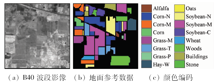
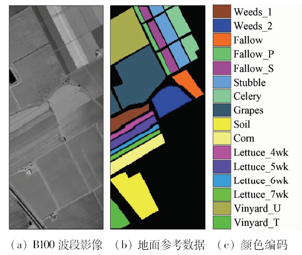
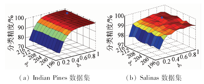
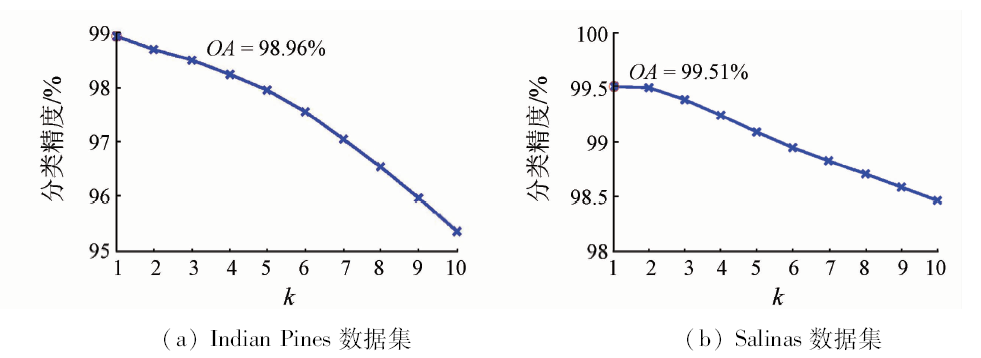
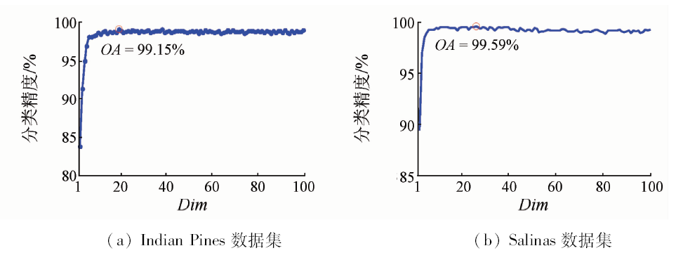
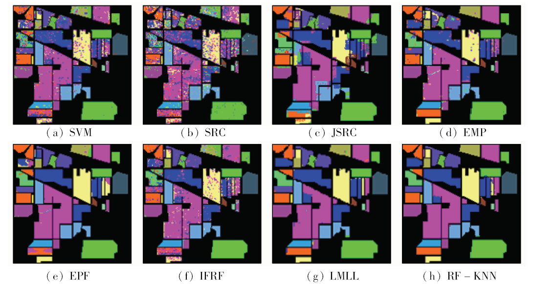
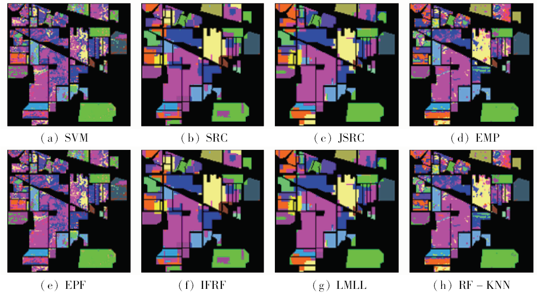
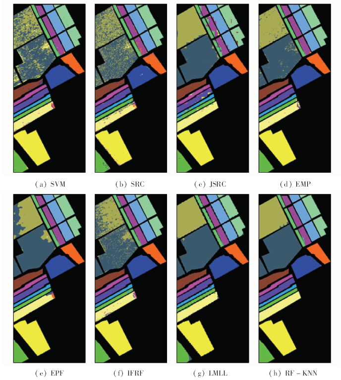
Abstract  

In order to remove the noise in the hyperspectral image effectively, strengthen the spatial structure, make full use of the spatial context information of the object, and improve the classification accuracy of hyperspectral image, the authors put forward recursive filtering and k-nearest neighbor (KNN) method for hyperspectral image classification. The main steps are as follows: Firstly, the principal component analysis (PCA) is used to perform feature dimension reduction of hyperspectral images. Next, the recursive filtering is used to filter the principal component image. Then, the Euclidean distance between the test sample and the different training samples is calculated by the KNN algorithm. Finally, according to the comparison of average values of k minimum Euclidean distances, the classification of test samples is achieved. Experimental results are based on several real-world hyperspectral data sets, and the influence of different parameters on the classification accuracy is analyzed. Experimental results show that, with recursive filtering, the noise can be effectively removed, and the image outline can be strengthened. Compared with other hyperspectral image classification methods, the proposed method is outstanding in classification accuracy.

Keywords hyperspectral images      recursive filtering      k-nearest neighbor      principal component analysis      Euclidean distance     
:  TP79  
Issue Date: 15 March 2019
Service
E-mail this article
E-mail Alert
RSS
Articles by authors
Bing TU
Xiaofei ZHANG
Guoyun ZHANG
Jinping WANG
Yao ZHOU
Cite this article:   
Bing TU,Xiaofei ZHANG,Guoyun ZHANG, et al. Hyperspectral image classification via recursive filtering and KNN[J]. Remote Sensing for Land & Resources, 2019, 31(1): 22-32.
URL:  
https://www.gtzyyg.com/EN/10.6046/gtzyyg.2019.01.04     OR     https://www.gtzyyg.com/EN/Y2019/V31/I1/22
Fig.1  Indian Pines data set
Fig.2  Salinas data set
Fig.3  Analysis of RF parameters on classification accuracy in different data sets
Fig.4  Analysis of the number of nearest neighbor on classification accuracy in different data sets
Fig.5  Analysis of dimension on classification accuracy in different data sets
Fig.6  Classification results of different algorithms in the Indian Pines data set (10% of training samples)
Fig.7  Classification results of different algorithms in the Indian Pines data set (1% of training samples)
指标 类别 训练样
本/个
测试样
本/个
SVM SRC JSRC EMP EPF IFRF LMLL RF-KNN
CA Alfalfa 10 36 79.31
(7.32)
61.58
(10.62)
94.44
(8.10)
94.44
(2.78)
97.86
(6.68)
99.73
(0.85)
94.44
(0.00)
94.44
(0.00)
Corn-N 143 1 285 78.49
(0.83)
53.06
(2.96)
93.81
(2.00)
87.77
(2.06)
95.95
(2.28)
97.55
(0.99)
94.75
(0.37)
98.49
(0.56)
Corn-M 83 747 80.74
(2.78)
50.33
(3.65)
91.51
(1.19)
92.74
(2.28)
96.00
(2.56)
98.59
(0.91)
73.76
(0.00)
98.69
(0.48)
Corn 34 203 67.72
(5.46)
37.56
(3.80)
91.74
(3.54)
85.73
(5.36)
92.21
(5.33)
97.62
(1.29)
98.59
(0.00)
99.70
(0.44)
Grass-M 48 435 90.28
(2.20)
83.77
(1.80)
92.37
(3.38)
92.00
(2.81)
99.00
(0.88)
98.96
(1.07)
95.86
(0.00)
97.33
(3.34)
Grass-T 23 707 89.28
(2.00)
91.39
(1.22)
93.55
(1.00)
97.63
(0.67)
95.15
(2.97)
99.05
(0.63)
100.00
(0.00)
96.94
(1.83)
Grass-P 15 13 83.04
(13.35)
82.00
(8.37)
100.00
(0.00)
94.44
(5.56)
97.24
(6.40)
91.43
(18.07)
100.00
(0.00)
100.00
(0.00)
Hay-W 28 450 97.47
(0.90)
93.30
(0.92)
99.02
(0.71)
99.91
(0.13)
99.99
(0.05)
100.00
(0.00)
100.00
(0.00)
100.00
(0.00)
Oats 15 5 46.35
(9.95)
55.00
(13.94)
62.00
(40.25)
100.00
(0.00)
100.00
(0.00)
81.82
(17.64)
100.00
(0.00)
100.00
(0.00)
Soybean-N 150 822 80.02
(2.17)
66.17
(3.90)
91.08
(1.93)
88.88
(0.78)
92.21
(4.48)
96.84
(1.35)
90.83
(0.00)
99.12
(0.89)
Soybean-M 246 2 209 80.84
(2.11)
70.16
(1.47)
97.08
(1.16)
95.38
(0.88)
91.71
(4.46)
98.07
(1.04)
91.67
(0.00)
99.29
(0.37)
Soybean-C 60 533 78.99
(3.24)
45.51
(2.62)
84.54
(4.64)
86.83
(2.37)
94.73
(3.60)
98.08
(1.07)
93.21
(0.34)
98.16
(0.98)
Wheat 21 184 93.80
(2.63)
91.74
(3.06)
86.20
(2.89)
99.24
(0.62)
100.00
(0.00)
97.60
(2.30)
99.46
(0.00)
99.02
(0.81)
Woods 127 1 138 91.96
(1.49)
89.19
(1.51)
99.51
(0.26)
99.63
(0.26)
95.11
(2.86)
99.70
(0.35)
97.98
(0.00)
99.72
(0.40)
Buildings 35 351 73.95
(4.28)
35.45
(1.85)
92.08
(4.33)
97.32
(1.69)
95.27
(2.64)
97.38
(1.69)
94.87
(0.00)
98.46
(1.47)
Stone 37 56 93.97
(4.13)
89.88
(2.64)
94.29
(4.96)
98.57
(0.80)
96.40
(3.11)
95.98
(5.05)
94.64
(0.00)
99.64
(0.80)
OA 83.33
(0.77)
68.47
(0.59)
94.19
(0.57)
94.41
(0.84)
94.47
(1.80)
98.23
(0.18)
94.45
(0.78)
98.82
(0.29)
AA 81.64
(1.30)
68.51
(1.89)
91.45
(1.27)
94.41
(0.84)
96.18
(0.89)
96.79
(1.80)
95.69
(0.51)
98.65
(0.33)
Kappa 80.90
(0.90)
64.02
(0.63)
93.37
(0.65)
92.77
(0.49)
93.67
(2.07)
97.98
(0.21)
93.65
(0.90)
98.69
(0.29)
Tab.1  Indian Pines data set classification accuracy of different algorithms (10% of training samples)
指标 类别 训练样
本/个
测试样
本/个
SVM SRC JSRC EMP EPF IFRF LMLL RF-KNN
CA Alfalfa 3 43 72.25
(5.43)
63.26
(18.20)
92.56
(9.21)
87.44
(6.41)
72.42
(30.15)
88.35
(31.74)
95.35
(0.00)
95.35
(0.00)
Corn-N 14 1 414 47.63
(7.37)
40.07
(5.91)
69.99
(6.50)
57.39
(4.59)
61.20
(8.91)
83.17
(8.34)
69.12
(0.42)
83.97
(10.41)
Corn-M 8 822 55.60
(15.51)
31.33
(6.92)
55.28
(8.60)
63.64
(7.29)
73.96
(18.37)
71.08
(10.79)
44.09
(0.11)
74.67
(14.06)
Corn 3 234 35.98
(11.21)
25.37
(8.55)
45.04
(15.61)
29.79
(9.89)
59.62
(33.29)
70.28
(12.62)
33.42
(0.19)
92.22
(8.31)
Grass-M 6 477 74.25
(12.10)
63.59
(10.07)
70.23
(26.81)
77.04
(9.38)
90.54
(12.56)
85.61
(9.82)
69.18
(0.00)
89.48
(3.16)
Grass-T 7 723 76.13
(6.57)
77.25
(8.63)
85.48
(3.41)
86.07
(13.92)
74.85
(6.53)
90.66
(5.52)
98.76
(0.00)
97.10
(1.64)
Grass-P 3 25 30.57
(15.22)
89.04
(5.76)
92.00
(12.33)
90.80
(9.25)
81.41
(30.42)
52.28
(25.97)
96.00
(0.00)
100.00
(0.00)
Hay-W 5 473 93.09
(5.37)
73.82
(12.02)
84.90
(8.79)
94.82
(3.02)
98.42
(2.99)
100.00
(0.00)
99.79
(0.00)
100.00
(0.00)
Oats 3 17 18.99
(9.95)
68.35
(20.16)
94.12
(10.19)
96.47
(7.44)
48.01
(37.62)
27.79
(20.58)
100.00
(0.00)
96.47
(7.89)
Soybean-N 10 962 53.88
(7.46)
49.04
(8.64)
71.10
(5.46)
69.27
(9.05)
70.51
(15.60)
72.87
(10.46)
73.80
(2.79)
84.30
(4.51)
Soybean-M 24 2 431 59.35
(4.18)
61.04
(4.71)
82.59
(5.06)
77.10
(6.22)
66.08
(9.18)
85.91
(4.45)
79.66
(0.13)
93.58
(4.15)
Soybean-C 6 587 38.95
(8.03)
21.85
(6.44)
48.07
(8.57)
39.93
(7.11)
56.11
(22.14)
70.91
(12.35)
55.54
(0.76)
80.20
(9.34)
Wheat 2 203 84.36
(4.03)
77.38
(11.01)
79.61
(12.27)
95.81
(1.89)
96.16
(3.87)
80.46
(12.73)
99.31
(0.44)
96.75
(2.38)
Woods 13 1 252 84.44
(2.87)
80.95
(6.80)
92.54
(7.27)
87.61
(5.30)
87.10
(5.07)
92.88
(1.76)
97.78
(0.04)
92,99
(6.50)
Buildings 4 382 42.01
(10.72)
19.04
(5.30)
36.70
(7.27)
61.52
(13.30)
67.86
(24.93)
80.08
(9.07)
20.37
(0.79)
83.66
(6.88)
Stone 3 90 96.89
(5.87)
87.00
(4.84)
96.89
(2.41)
71.44
(25.08)
93.81
(20.70)
97.97
(10.17)
74.89
(1.49)
98.67
(0.93)
OA 60.60
(2.00)
54.87
(1.63)
74.04
(1.37)
71.88
(2.25)
71.00
(2.97)
81.84
(2.88)
86.72
(5.32)
89.07
(1.17)
AA 57.46
(2.63)
58.02
(2.14)
74.82
(2.74)
74.13
(3.18)
74.88
(5.28)
78.14
(3.00)
84.91
(4.79)
87.57
(1.32)
Kappa 54.59
(2.16)
48.47
(1.86)
70.12
(1.52)
67.88
(2.52)
66.24
(3.70)
79.29
(3.28)
84.77
(6.11)
91.21
(0.84)
Tab.2  Indian Pines data set classification accuracy of different algorithms (1% of training samples)
Fig.8  Classification results of different algorithms in the Salinas data set (2% of training samples)
Fig. 9  Classification results of different algorithms in the Salinas data set (0.2% of training samples)
指标 类别 训练样
本/个
测试样
本/个
SVM SRC JSRC EMP EPF IFRF LMLL RF-KNN
CA Weeds_1 40 1 969 100.00
(0.00)
98.36
(0.65)
100.00
(0.00)
99.80
(0.00)
100.00
(0.00)
100.00
(0.00)
100.00
(0.00)
100.00
(0.00)
Weeds_2 73 3 653 97.19
(0.53)
98.52
(0.45)
99.41
(0.67)
99.56
(0.34)
100.00
(0.00)
99.99
(0.02)
100.00
(0.00)
99.86
(0.13)
Fallow 38 1 938 94.60
(1.45)
96.76
(1.21)
99.16
(0.77)
99.54
(0.27)
94.84
(1.61)
99.88
(0.08)
99.69
(0.15)
100.00
(0.00)
Fallow_P 26 1 368 97.63
(1.11)
99.26
(0.33)
88.67
(5.45)
98.30
(1.20)
98.02
(0.56)
97.84
(0.92)
98.26
(2.88)
97.35
(2.34)
Fallow_S 52 2 626 98.55
(0.54)
94.39
(0.68)
84.03
(2.06)
96.77
(0.46)
99.94
(0.05)
99.47
(0.98)
99.06
(0.28)
98.64
(0.89)
Stubble 79 3 880 99.97
(0.05)
99.69
(0.10)
98.20
(1.33)
99.60
(0.38)
99.98
(0.02)
100.00
(0.00)
100.00
(0.00)
99.76
(0.18)
Celery 70 3 509 99.40
(0.31)
99.27
(0.14)
95.10
(2.08)
99.58
(0.09)
99.84
(0.17)
99.81
(0.11)
99.94
(0.00)
99.93
(0.05)
Graps 225 11 046 74.60
(1.74)
73.62
(1.49)
98.47
(0.23)
96.38
(0.91)
84.10
(4.04)
99.64
(0.14)
92.72
(0.06)
99.87
(0.19)
Soil 124 6 079 99.62
(0.03)
97.89
(0.93)
99.99
(0.01)
99.84
(0.23)
99.18
(0.32)
99.92
(0.12)
100.00
(0.00)
100.00
(0.00)
Corn 21 3 257 79.07
(5.21)
78.13
(3.72)
89.60
(3.36)
93.38
(1.17)
99.21
(0.83)
99.64
(0.42)
89.72
(1.99)
98.66
(0.73)
Lettuce_4wk 21 1 047 86.93
(4.99)
96.58
(2.71)
88.83
(4.86)
96.85
(1.53)
96.97
(1.27)
99.20
(0.30)
95.52
(0.77)
97.06
(2.52)
Lettuce_5wk 38 1 889 97.96
(0.49)
99.72
(0.58)
94.55
(0.99)
99.52
(0.98)
99.46
(0.63)
98.82
(1.22)
100.00
(0.00)
99.68
(0.40)
Lettuce_6wk 18 898 98.47
(0.85)
97.34
(0.43)
83.78
(5.46)
98.57
(1.17)
98.58
(1.62)
99.01
(1.22)
97.16
(0.13)
91.76
(8.28)
Lettuce_7wk 20 1 050 86.93
(4.81)
92.69
(2.17)
79.62
(5.57)
96.13
(1.75)
98.71
(0.53)
98.16
(1.25)
97.52
(0.04)
98.84
(0.66)
Vinyard_U 140 7 128 66.51
(5.39)
61.41
(1.96)
97.39
(0.47)
94.23
(1.16)
91.82
(2.37)
99.88
(0.16)
68.43
(1.31)
99.01
(0.44)
Vinyard_T 36 1 771 96.88
(2.12)
95.57
(2.75)
99.64
(0.18)
99.31
(0.39)
99.75
(0.44)
99.97
(0.05)
97.33
(0.48)
100.00
(0.00)
OA 87.57
(1.08)
86.69
(0.54)
95.98
(0.53)
97.53
(0.20)
94.78
(1.23)
99.42
(0.10)
93.23
(0.19)
99.46
(0.12)
AA 92.14
(0.85)
92.45
(0.54)
93.53
(1.09)
97.96
(0.25)
97.53
(0.32)
99.15
(0.10)
95.95
(0.21)
99.29
(0.14)
Kappa 86.14
(1.19)
85.17
(0.61)
95.53
(0.59)
97.25
(0.22)
94.17
(1.38)
99.62
(0.11)
92.44
(0.21)
98.78
(0.54)
Tab.3  Salinas data set classification accuracy of different algorithms (2% of training samples)
指标 类别 训练样
本/个
测试样
本/个
SVM SRC JSRC EMP EPF IFRF LMLL RF-KNN
CA Weeds_1 4 2 005 99.97
(0.04)
96.22
(1.21)
100.00
(0.00)
95.22
(9.57)
100.00
(0.00)
95.83
(5.08)
99.56
(0.41)
94.54
(8.02)
Weeds_2 8 3 718 94.87
(5.09)
97.60
(1.88)
99.70
(0.32)
98.95
(0.47)
99.96
(0.08)
99.77
(0.49)
99.74
(0.13)
99.09
(3.72)
Fallow 4 1 972 86.58
(4.53)
81.85
(13.07)
92.11
(9.31)
75.79
(17.54)
88.15
(1.26)
98.00
(2.63)
99.62
(0.18)
100.00
(0.00)
Fallow_P 3 1 391 97.17
(0.48)
99.07
(0.49)
56.96
(18.30)
99.01
(0.53)
97.47
(0.62)
91.10
(8.78)
56.70
(2.61)
76.62
(8.58)
Fallow_S 5 2 673 97.94
(0.80)
90.47
(4.61)
79.07
(6.65)
94.52
(2.44)
93.95
(7.58)
98.54
(2.22)
99.13
(0.38)
93.52
(4.98)
Stubble 8 3 951 99.98
(0.06)
99.59
(0.10)
99.83
(0.14)
97.05
(2.45)
99.97
(0.04)
100.00
(0.00)
99.52
(0.21)
97.77
(1.28)
Celery 7 3 572 95.19
(3.65)
98.55
(1.62)
96.41
(1.60)
99.34
(0.21)
97.79
(3.06)
99.39
(0.69)
99.73
(0.09)
98.64
(1.49)
Graps 21 11 250 64.31
(4.69)
69.24
(5.61)
89.36
(2.82)
85.68
(7.31)
70.03
(7.78)
95.22
(5.66)
88.20
(1.35)
93.77
(4.58)
Soil 11 6 192 99.59
(0.03)
96.97
(0.59)
99.61
(0.67)
99.26
(0.64)
92.56
(10.95)
98.58
(3.35)
99.01
(1.16)
100.00
(0.00)
Corn 3 3 275 77.73
(8.42)
54.75
(20.40)
79.57
(1.88)
73.97
(16.68)
91.63
(4.47)
98.94
(0.70)
90.02
(3.62)
97.92
(1.69)
Lettuce_4wk 3 1 065 64.29
(6.73)
93.12
(3.49)
80.56
(9.38)
94.80
(1.60)
76.28
(28.19)
98.75
(0.40)
92.94
(0.75)
88.26
(5.87)
Lettuce_5wk 4 1 923 92.36
(3.56)
97.32
(3.13)
71.45
(13.17)
99.95
(0.12)
96.28
(6.13)
92.19
(3.75)
100.00
(0.00)
80.09
(14.87)
Lettuce_6wk 2 914 89.61
(10.32)
97.19
(1.66)
56.09
(13.08)
98.49
(0.44)
86.04
(8.46)
83.58
(16.15)
97.55
(0.65)
71.66
(19.57)
Lettuce_7wk 2 1 068 71.56
(18.02)
81.08
(4.11)
94.41
(1.47)
92.57
(3.86)
98.83
(0.77)
81.37
(17.11)
96.66
(1.97)
60.28
(22.83)
Vinyard_U 13 7 255 45.34
(4.69)
53.50
(6.93)
70.38
(8.04)
72.99
(8.62)
87.61
(10.47)
89.90
(6.73)
72.37
(2.60)
96.61
(1.49)
Vinyard_T 4 1 803 93.56
(10.78)
73.55
(11.52)
96.14
(4.08)
86.88
(8.76)
99.93
(0.09)
99.63
(1.17)
96.04
(5.00)
99.80
(0.45)
OA 79.33
(1.99)
81.14
(1.39)
87.44
(1.02)
89.32
(2.00)
86.23
(2.51)
94.40
(2.08)
91.48
(0.87)
94.93
(1.26)
AA 85.63
(1.86)
86.25
(1.21)
85.10
(0.88)
91.53
(1.38)
92.28
(1.89)
94.05
(1.98)
92.93
(0.91)
94.69
(1.40)
Kappa 77.14
(2.15)
78.97
(1.52)
85.99
(1.14)
88.08
(2.22)
84.55
(2.88)
94.18
(2.32)
90.50
(0.97)
94.41
(3.05)
Tab.4  Salinas data set classification accuracy of different algorithms (0.2% of training samples)
[1] 王跃明, 郎均慰, 王建宇 . 航天高光谱成像技术研究现状及展望[J]. 激光与光电子学进展, 2013,50(1):75-82.
doi: 10.3788/LOP50.010008 url: http://www.cnki.com.cn/Article/CJFDTotal-JGDJ201301009.htm
[1] Wang Y M, Lang J W, Wang J Y . Status and prospect of space-borne hyperspectral imaging technology[J]. Laser and Optoelectronics Progress, 2013,50(1):75-82.
[2] Manolakis D, Shaw G . Detection algorithms for hyperspectral imaging applications[J]. IEEE Signal Processing Magazine, 2002,19(1):29-43.
doi: 10.1109/79.974724 url: http://ieeexplore.ieee.org/document/974724/
[3] Bioucas-Dias J M, Plaza A, Camps-Valls G , et al. Hyperspectral remote sensing data analysis and future challenges[J]. IEEE Geoscience and Remote Sensing Magazine, 2013,1(2):6-36.
doi: 10.1109/MGRS.2013.2244672 url: http://ieeexplore.ieee.org/xpls/icp.jsp?arnumber=6555921
[4] 李庆亭, 张连蓬, 杨锋杰 , 等. 高光谱遥感图像最大似然分类问题及解决方法[J]. 山东科技大学学报(自然科学版), 2005,24(3):61-64.
doi: 10.3969/j.issn.1672-3767.2005.03.017 url: http://www.cnki.com.cn/Article/CJFDTotal-SDKY200503016.htm
[4] Li Q T, Zhang L P, Yang F J , et al. The MLC’s problem in classification of hyperspectral RS image and its solving method[J]. Journal of Shandong University of Science (Natural Science Edition), 2005,24(3):61-64.
[5] Melgani F, Bruzzone L . Classification of hyperspectral remote sensing images with support vector machines[J]. IEEE Transactions on Geoscience and Remote Sensing, 2004,42(8):1778-1790.
doi: 10.1109/TGRS.2004.831865 url: http://ieeexplore.ieee.org/document/1323134/
[6] Fauvel M, Tarabalka Y, Benediktsson J A , et al. Advances in spectral-spatial classification of hyperspectral images[J]. Proceedings of the IEEE Transactions on Geoscience and Remote Sensing, 2013,101(3):652-675.
doi: 10.1109/JPROC.2012.2197589 url: http://ieeexplore.ieee.org/document/6297992
[7] 王春瑶, 陈俊周, 李炜 . 超像素分割算法研究综述[J]. 计算机应用研究, 2014,31(1):6-12.
doi: 10.3969/j.issn.1001-3695.2014.01.002 url: http://www.cqvip.com/QK/93231X/201401/48243238.html
[7] Wang C Y, Chen J Z, Li W . Review on superpixel segmentation algorithms[J]. Application Research of Computers, 2014,31(1):6-12.
[8] 彭海涛, 柯长青 . 基于多层分割的面向对象遥感影像分类方法研究[J]. 遥感技术与应用, 2010,25(1):149-154.
url: http://d.wanfangdata.com.cn/Periodical/ygjsyyy201001024
[8] Peng H T, Ke C Q . Study on object-oriented remote sensing image classification based on multi-levels segmentation[J]. Remote Sensing Technology and Application, 2010,25(1):149-154.
[9] Vincent L, Soille P . Watersheds in digital spaces:An efficient algorithm based on immersion simulations[J]. IEEE Transactions on Pattern Analysis and Machine Intelligence, 1991,13(6):583-598.
doi: 10.1109/34.87344 url: http://ieeexplore.ieee.org/document/87344/
[10] 王亚静, 王正勇, 滕奇志 , 等. 基于熵率超像素和区域合并的岩屑颗粒图像分割[J].计算机工程与设计, 2014(12):4223-4227.
doi: 10.3969/j.issn.1000-7024.2014.12.032 url: http://d.wanfangdata.com.cn/Periodical/jsjgcysj201412032
[10] Wang Y J, Wang Z Y, Teng Q Z , et al. Image segmentation of cutting grains based on entropy rate superpixel and region merging[J].Computer Engineering and Design, 2014(12):4223-4227.
[11] 李旭超, 朱善安 . 图像分割中的马尔可夫随机场方法综述[J]. 中国图象图形学报, 2007,12(5):789-798.
doi: 10.3969/j.issn.1006-8961.2007.05.004 url: http://d.wanfangdata.com.cn/Periodical/zgtxtxxb-a200705004
[11] Li X C, Zhu S A . A survey of the Markov random field method for image segmentation[J]. Journal of Image and Graphics, 2007,12(5):789-798.
[12] Tarabalka Y Chanussot J, Benediktsson J A . Segmentation and classification of hyperspectral images using minimum spanning forest grown from automatically selected markers[J]. IEEE Transactions on Systems,Man,and Cybernetics.Part B,Cybernetics:A Publication of the IEEE Systems,Man,and Cybernetics Society, 2010,40(5):1267-1279.
doi: 10.1109/TSMCB.2009.2037132 pmid: 20051346 url: http://ieeexplore.ieee.org/document/5371866/
[13] 马秀丹, 吴子宾 . 一种优化的高光谱图像特征提取方法[J].河南科技, 2016(9):29-30.
doi: 10.3969/j.issn.1003-5168.2016.09.008 url: http://d.wanfangdata.com.cn/Periodical/hnkj201609008
[13] Ma X D, Wu Z B . An optimization feature extraction method of hyperspectral images[J].Journal of Henan Science and Technology, 2016(9):29-30.
[14] 朱勇, 吴波 . 多相似测度稀疏表示的高光谱影像分类[J]. 遥感信息, 2016,31(4):9-15.
doi: 10.3969/j.issn.1000-3177.2016.04.002 url: http://www.cnki.com.cn/Article/CJFDTotal-YGXX201604002.htm
[14] Zhu Y, Wu B . Sparse representation classification of hyperspectral image based on similarity indices[J]. Remote Sensing Information, 2016,31(4):9-15.
[15] 程志会, 谢福鼎 . 基于空间特征与纹理信息的高光谱图像半监督分类[J].测绘通报, 2016(12):56-59,73.
doi: 10.13474/j.cnki.11-2246.2016.0401 url: http://www.cqvip.com/QK/93318X/201612/670895035.html
[15] Cheng Z H, Xie F D . Semi-supervised classification for hyperspectral image based on spatial features and texture information[J].Bulletin of Surveying and Mapping, 2016(12):56-59,73.
[16] 张朝阳, 冯伍法, 张俊华 , 等. 基于形态学色差的彩色遥感影像水域提取[J]. 海洋测绘, 2006,26(5):58-60.
doi: 10.3969/j.issn.1671-3044.2006.05.018 url: http://d.wanfangdata.com.cn/Periodical/hych200605018
[16] Zhang Z Y, Feng W F, Zhang J H , et al. The waters feature extraction from the RS color image based on the morphological chromatic aberration[J]. Hydrographic Surveying and Charting, 2006,26(5):58-60.
[17] Camps-Valls G, Gomez-Chova L, Munoz-Mari J , et al. Composite kernels for hyperspectral image classification[J]. IEEE Geoscience and Remote Sensing Letters, 2006,3(1):93-97.
doi: 10.1109/LGRS.2005.857031 url: http://ieeexplore.ieee.org/document/1576697/
[18] Zhang L F, Zhang L P, Tao D C , et al. On combining multiple features for hyperspectral remote sensing image classification[J]. IEEE Transactions on Geoscience and Remote Sensing, 2012,50(3):879-893.
doi: 10.1109/tgrs.2011.2162339 url: http://ieeexplore.ieee.org/document/5997309/
[19] Kang X D, Li S T, Benediktsson J A . Feature extraction of hyperspectral images with image fusion and recursive filtering[J]. IEEE Transactions on Geoscience and Remote Sensing, 2014,52(6):3742-3752.
doi: 10.1109/TGRS.2013.2275613 url: http://ieeexplore.ieee.org/document/6600779/
[20] Wang Z W, Yang J C, Nasrabadi N, et al. A max-margin perspective on sparse representation-based classification [C]//IEEE International Conference on Computer Vision.Sydney:IEEE, 2013: 1217-1224.
[21] Chen Y, Nasrabadi N M, Tran T D . Hyperspectral image classification using dictionary-based sparse representation[J]. IEEE Transactions on Geoscience and Remote Sensing, 2011,49(10):3973-3985.
doi: 10.1109/TGRS.2011.2129595 url: http://ieeexplore.ieee.org/document/5766028/
[22] Benediktsson J A, Palmason J A, Sveinsson J R . Classification of hyperspectral data from urban areas based on extended morphological profiles[J]. IEEE Transactions on Geoscience and Remote Sensing, 2005,43(3):480-491.
doi: 10.1109/TGRS.2004.842478 url: http://ieeexplore.ieee.org/document/1396321/
[23] Kang X D, Li S T, Benediktsson J A . Spectral-spatial hyperspectral image classification with edge-preserving filtering[J]. IEEE Transactions on Geoscience and Remote Sensing, 2014,52(5):2666-2677.
doi: 10.1109/TGRS.2013.2264508 url: http://ieeexplore.ieee.org/document/6553593/
[24] Li J ,Bioucas-Dias J M,Plaza A.Hyperspectral image segmentation using a new Bayesian approach with active learning[J]. IEEE Transactions on Geoscience and Remote Sensing, 2011,49(10):3947-3960.
doi: 10.1109/TGRS.2011.2128330 url: http://ieeexplore.ieee.org/document/5766734/
[1] QIN Dahui, YANG Ling, CHEN Lunchao, DUAN Yunfei, JIA Hongliang, LI Zhenpei, MA Jianqin. A study on the characteristics and model of drought in Xinjiang based on multi-source data[J]. Remote Sensing for Natural Resources, 2022, 34(1): 151-157.
[2] ZHANG Qinrui, ZHAO Liangjun, LIN Guojun, WAN Honglin. Ecological environment assessment of three-river confluence in Yibin City using improved remote sensing ecological index[J]. Remote Sensing for Natural Resources, 2022, 34(1): 230-237.
[3] GAO Wenlong, ZHANG Shengwei, LIN Xi, LUO Meng, REN Zhaoyi. The remote sensing-based estimation and spatial-temporal dynamic analysis of SOM in coal mining[J]. Remote Sensing for Natural Resources, 2021, 33(4): 235-242.
[4] WEI Yingjuan, LIU Huan. Remote sensing-based mineralized alteration information extraction and prospecting prediction of the Beiya gold deposit, Yunnan Province[J]. Remote Sensing for Natural Resources, 2021, 33(3): 156-163.
[5] WU Yu, ZHANG Jun, LI Yixu, HUANG Kangyu. Research on building cluster identification based on improved U-Net[J]. Remote Sensing for Land & Resources, 2021, 33(2): 48-54.
[6] CHEN Zhen, XIA Xueqi, CHEN Jianping. A study of remote sensing evaluation model and main controlling factors of land ecological quality:A case study of Guang’an City[J]. Remote Sensing for Land & Resources, 2021, 33(1): 191-198.
[7] MUHADAISI Ariken, ZHANG Fei, LIU Kang, AYINUER Yushanjiang. Urban ecological environment evaluation based on Tiangong-2 and Landsat8 data[J]. Remote Sensing for Land & Resources, 2020, 32(4): 209-218.
[8] Benzuo YAO, Fang HE. Spatial and spectral feature hierarchical fusion for hyperspectral image feature extraction[J]. Remote Sensing for Land & Resources, 2019, 31(3): 59-64.
[9] Ruhan A, Fang HE, Biaobiao WANG. Hyperspectral images classification via weighted spatial-spectral dimensionality reduction principle component analysis[J]. Remote Sensing for Land & Resources, 2019, 31(2): 17-23.
[10] Lixin DONG. Multi-model estimation of forest leaf area index in the Three Gorges Reservoir area[J]. Remote Sensing for Land & Resources, 2019, 31(2): 73-81.
[11] Sirui YANG, Zhaohui XUE, Ling ZHANG, Hongjun SU, Shaoguang ZHOU. Fusion of hyperspectral and LiDAR data: A case study for refined crop classification in agricultural region of Zhangye Oasis in the middle reaches of Heihe River[J]. Remote Sensing for Land & Resources, 2018, 30(4): 33-40.
[12] Lingyu YIN, Xianlin QIN, Guifen SUN, Shuchao LIU, Xiaofeng ZU, Xiaozhong CHEN. The method for detecting forest cover change in GF-1images by using KPCA[J]. Remote Sensing for Land & Resources, 2018, 30(1): 95-101.
[13] Hongmin ZHANG, Yanfang ZHANG, Mao TIAN, Chunling WU. Dynamic monitoring of eco-environment quality changes based on PCA:A case study of urban area of Baoji City[J]. Remote Sensing for Land & Resources, 2018, 30(1): 203-209.
[14] ZHANG Qianning, TAN Shiteng, XU Zhu, HUANG Zechun. Applicability and simplification study of patch level landscape metrics based on GLC30[J]. REMOTE SENSING FOR LAND & RESOURCES, 2017, 29(4): 98-105.
[15] DONG Anguo, GONG Wenjuan, HAN Xue. Band selection method for hyperspectral image based on linear representation[J]. REMOTE SENSING FOR LAND & RESOURCES, 2017, 29(4): 39-42.
Viewed
Full text


Abstract

Cited

  Shared   
  Discussed   
京ICP备05055290号-2
Copyright © 2017 Remote Sensing for Natural Resources
Support by Beijing Magtech