|
|
 |
|

|
|
|
Principal component selection method for hyperspectral remote sensing images based on spatial statistics |
SUN Xiao1( ), PENG Junhuan2(), ZHAO Feng3, WANG Xiaoyang1, LYU Jie2, ZHANG Dengfeng4 ), PENG Junhuan2(), ZHAO Feng3, WANG Xiaoyang1, LYU Jie2, ZHANG Dengfeng4 |
1. Langfang Natural Resources Comprehensive Survey Center, China Geological Survey, Langfang 065000, China
2. School of Land Science and Technology, China University of Geosciences (Beijing), Beijing 100083, China
3. Urumqi Natural Resources Comprehensive Survey Center, China Geological Survey, Urumqi 830057, China
4. Xi’an Center of Mineral Resources Survey, China Geological Survey, Xi’an 710100, China |
|
|
|
|
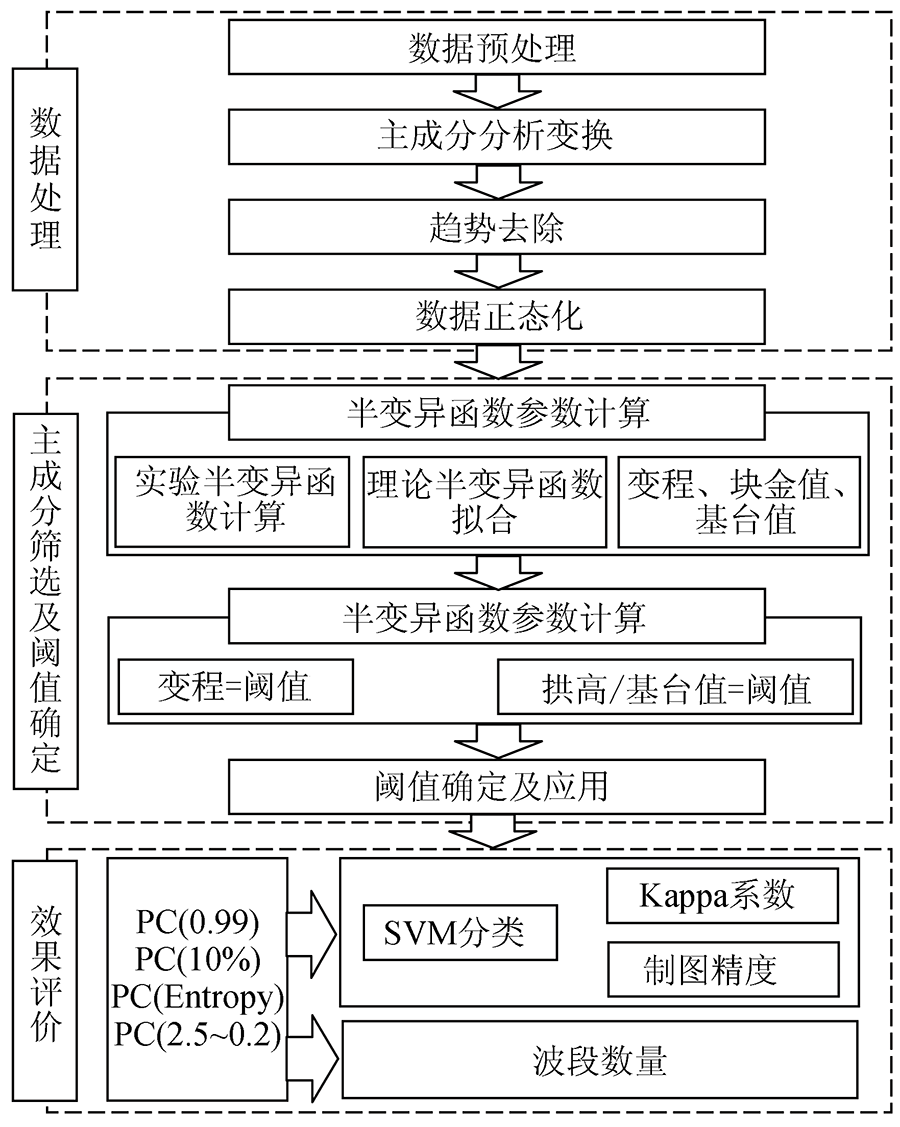
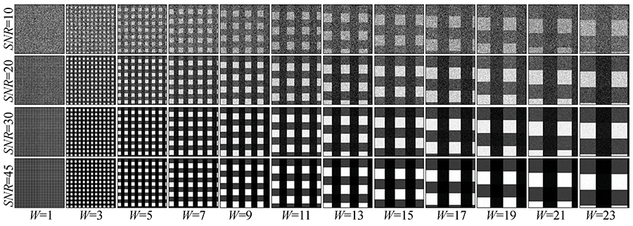
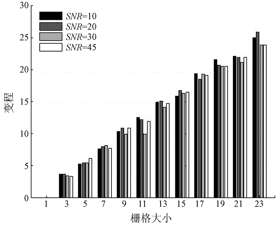
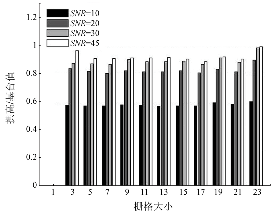
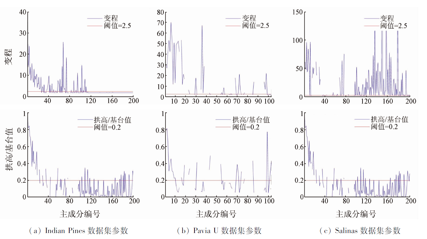
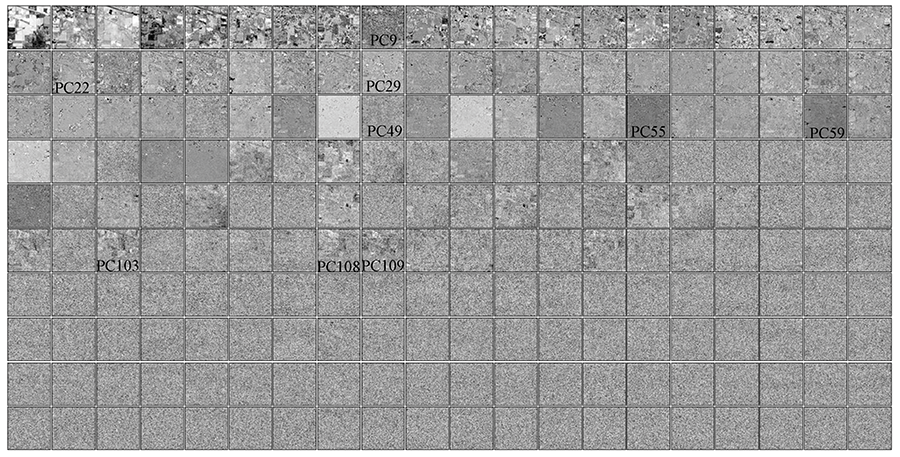
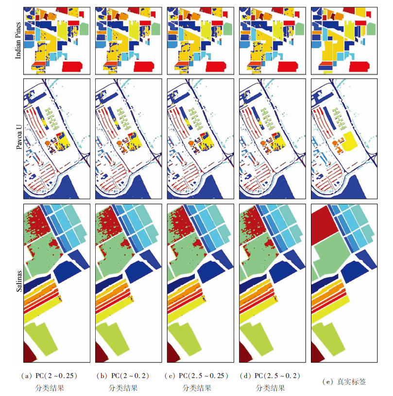
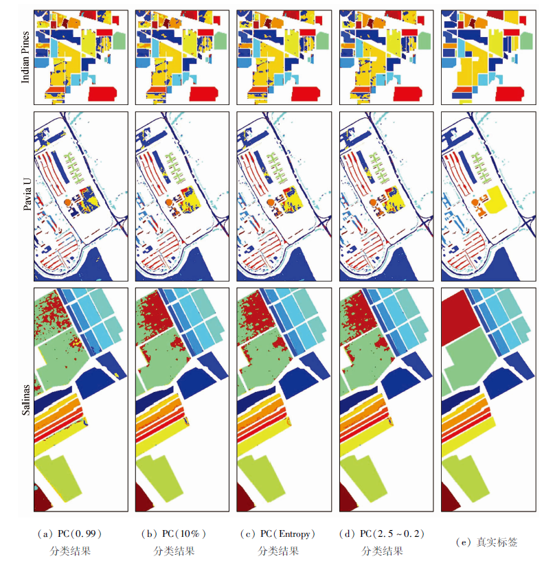
Abstract The principal component analysis is a widely used method for dimensionality reduction of hyperspectral remote sensing images. In task-oriented work, the principal component selection method based on cumulative variance contribution rate is not ideal. To address the problem of principal component selection after principal component analysis transformation, a method of principal component selection based on spatial statistics is proposed. The selection of principal components is performed by calculating the values of the semi-variogram parameter range and partial sill/sill of each principal component. The magnitude of a range is used to judge the range of spatial correlation of each principal component, and the partial sill/sill is used to judge the strength of spatial correlation of each principal component. The simulation proves that the variable range and partial sill/sill can effectively express the range and strength of spatial correlation of hyperspectral remote sensing images. Based on the experiment of real hyperspectral remote sensing images, the empirical threshold of principal component selection is determined from subjective and objective aspects, that is, the range is 2.5, and the partial sill/sill is 0.2. According to the classification results based on the support vector machine algorithm, compared with traditional methods, the principal components with better image quality can be screened by using variable range and partial sill/sill, which can not only achieve the purpose of dimensionality reduction, but also ensure high classification accuracy.
|
| Keywords
hyperspectral
principal component analysis
spatial statistics
semi-variogram
support vector machine
|
|
|
|
Corresponding Authors:
PENG Junhuan
E-mail: sunxiao@mail.cgs.gov.cn;pengjunhuan@163.com
|
|
Issue Date: 20 June 2022
|
|
|
| [1] |
Hughes G. On the mean accuracy of statistical pattern recognizers[J]. IEEE Transactions on Information Theory, 1968, 14(1):55-63.
doi: 10.1109/TIT.1968.1054102
url: http://ieeexplore.ieee.org/document/1054102/
|
| [2] |
Chang C-I. Hyperspectral Data Exploitation:Theory and Applications[M]. John Wiley & Sons Inc,Hoboken,New Jersey, 2007,205.
|
| [3] |
宋海峰, 陈广胜, 杨巍巍. 基于PCA的高光谱遥感图像分类[J]. 测绘工程, 2017, 26(12):17-20,26.
|
| [3] |
Song H F, Chen G S, Yang W W. Principal component analysis for hyper spectral image classification[J]. Engineering of Surveying and Mapping, 2017, 26(12):17-20,26.
|
| [4] |
Jolliffe I T. Principal Component Analysis[M]. Wiley, 2nd edition, 2002.
|
| [5] |
Pu R, Gong P, Tian Y, et al. Invasive species change detection using artificial neural networks and CASI hyperspectral imagery[J]. Environmental Monitoring and Assessment, 2008, 140(1-3):15-32.
doi: 10.1007/s10661-007-9843-7
url: http://link.springer.com/10.1007/s10661-007-9843-7
|
| [6] |
Chen G, Qian S. Denoising and dimensionality reduction of hyperspectral imagery using wavelet packets,neighbour shrinking and principal component analysis[J]. International Journal of Remote Sensing, 2009, 30(18):4889-4895.
doi: 10.1080/01431160802653724
url: https://www.tandfonline.com/doi/full/10.1080/01431160802653724
|
| [7] |
Canty M J, Nielsen A A. Linear and kernel methods for multivariate change detection[J]. Computers & Geosciences, 2012, 38(1):107-114.
doi: 10.1016/j.cageo.2011.05.012
url: https://linkinghub.elsevier.com/retrieve/pii/S0098300411001889
|
| [8] |
Foca G, Ferrari C, Ulrici A, et al. The potential of spectral and hyperspectral-imaging techniques for bacterial detection in food:A case study on lactic acid bacteria[J]. Talanta, 2016, 2016(153):111-119.
|
| [9] |
Li B, Hou B, Zhang D, et al. Pears characteristics (soluble solids content and firmness prediction,varieties) testing methods based on visible-near infrared hyperspectral imaging[J]. Optik International Journal for Light and Electron Optics, 2016, 127(5):2624-2630.
doi: 10.1016/j.ijleo.2015.11.193
url: https://linkinghub.elsevier.com/retrieve/pii/S0030402615018264
|
| [10] |
韩彦岭, 崔鹏霞, 杨树瑚, 等. 基于残差网络特征融合的高光谱图像分类[J]. 国土资源遥感, 2021, 33(2):11-19.doi: 10.6046/gtzyyg.2020209.
doi: 10.6046/gtzyyg.2020209
|
| [10] |
Han Y L, Gui P X, Yang S H, et al. Classification of hyperspectral image based on feature fusion of residual network[J]. Remote Sensing for Land and Resources, 2021, 33(2):11-19.doi: 10.6046/gtzyyg.2020209.
doi: 10.6046/gtzyyg.2020209
|
| [11] |
Chang Y, Wang Y, Liu T, et al. Fault diagnosis of a mine hoist using PCA and SVM techniques[J]. Journal of China University of Mining and Technology, 2008, 18(3):327-331.
doi: 10.1016/S1006-1266(08)60069-3
url: https://linkinghub.elsevier.com/retrieve/pii/S1006126608600693
|
| [12] |
Li C, Liu L, Lei Y, et al. Clustering for HSI hyperspectral image with weighted PCA and ICA[J]. Journal of Intelligent & Fuzzy Systems:Applications in Engineering and Technology, 2017, 32(5):3729-3737.
|
| [13] |
臧卓, 林辉, 杨敏华. 利用PCA算法进行乔木树种高光谱数据降维与分类[J]. 测绘科学, 2014, 188(2):146-149.
|
| [13] |
Zang Z, Lin H, Yang M H. Dimension reduction and classification of hyperspectral data of tree species using PCA algorithm[J]. Science of Surveying and Mapping, 2014, 188(2):146-149.
|
| [14] |
黄鸿, 曲焕鹏. 基于半监督稀疏鉴别嵌入的高光谱遥感影像分类[J]. 光学精密工程, 2014, 22(2):434-442.
|
| [14] |
Huang H, Qu H P. Hyperspectral remote sensing image classification based on SSDE[J]. Optics and Precision Engineering, 2014, 22(2):434-442.
doi: 10.3788/OPE.20142202.0434
url: http://www.opticsjournal.net/Abstract.htm?id=OJ140303000183D0FcIf
|
| [15] |
Lee C, Youn S, Jeong T, et al. Hybrid compression of hyperspectral images based on PCA with pre-encoding discriminant information[J]. IEEE Geoscience and Remote Sensing Letters, 2015, 12(7):1491-1495.
doi: 10.1109/LGRS.2015.2409897
url: http://ieeexplore.ieee.org/document/7063895/
|
| [16] |
袁林, 胡少兴, 张爱武, 等. 基于深度学习的高光谱图像分类方法[J]. 人工智能与机器人研究, 2017, 6(1):31-39.
|
| [16] |
Yuan L, Hu S X, Zhang A W, et al. A classification method for hyperspectral imagery based on deep learning[J]. Artificial Intelligence and Robotics Research, 2017, 6(1):31-39.
doi: 10.12677/AIRR.2017.61005
url: http://www.HansPub.org/journal/PaperDownload.aspx?DOI=10.12677/AIRR.2017.61005
|
| [17] |
臧卓, 林辉, 杨敏华. ICA与PCA在高光谱数据降维分类中的对比研究[J]. 中南林业科技大学学报, 2011, 31(11):18-22.
|
| [17] |
Zang Z, Lin H, Yang M H. Comparative study on descending dimension classification of hyperspectral data between ICA algorithm and PCA algorithm[J]. Journal of Central South University of Forestry & Technology, 2011, 31(11):18-22.
|
| [18] |
叶珍, 何明一. PCA与移动窗小波变换的高光谱决策融合分类[J]. 中国图象图形学报, 2015, 20(1):132-139.
|
| [18] |
Ye Z, He M Y. PCA and windowed wavelet transform for hyperspectral decision fusion classification[J]. Journal of Image and Graphics, 2015, 20(1):132-139.
|
| [19] |
Abdolmaleki M, Fathianpour N, Tabaei M. Evaluating the performance of the wavelet transform in extracting spectral alteration features from hyperspectral images[J]. International Journal of Remote Sensing, 2018, 2018:1-19.
|
| [20] |
Mather P, Koch M. Computer processing of remotely-sensed images[M]. John Wiley & Sons,Ltd, 2011,265.
|
| [21] |
Rodarmel C, Shan J. Principal component analysis for hyperspectral image classification[J]. Surveying and Land Information Systems, 2002, 62(2):115-122.
|
| [22] |
Ibarrola-Ulzurrun E, Marcello J, Gonzalo-Martin C. Assessment of component selection strategies in hyperspectral imagery[J]. Entropy, 2017, 19:1-17.
doi: 10.3390/e19010001
url: http://www.mdpi.com/1099-4300/19/1/1
|
| [23] |
Stephan K, Hibbitts C, Hoffmann H, et al. Reduction of instrument-dependent noise in hyperspectral image data using the principal component analysis:Applications to Galileo NIMS data[J]. Planetary and Space Science, 2008, 56(3-4):406-419.
doi: 10.1016/j.pss.2007.11.021
url: https://linkinghub.elsevier.com/retrieve/pii/S0032063307003613
|
| [24] |
Zheng W, Lai J, Yuen P. GA-Fisher:A new LDA-based face recognition algorithm with selection of principal components[J]. IEEE Transactions on Systems,Man and Cybernetics,Part B (Cybernetics), 2005, 35(5):1065-1078.
doi: 10.1109/TSMCB.2005.850175
url: http://ieeexplore.ieee.org/document/1510780/
|
| [25] |
Zhang X, Li R, Jiao L. Feature extraction combining PCA and immune clonal selection for hyperspectral remote sensing image classification[C]. International Conference on Artificial Intelligence & Computational Intelligence,IEEE, 2009.
|
| [26] |
Tobler W. Cellular geography[M]. Springer Netherlands, 1979,379-386.
|
| [27] |
戴平生, 陈建宝. 空间统计学研究应用综述[C]// 烟台: 国际应用统计学术研讨会, 2008.
|
| [27] |
Dai P S, Chen J B. Review of spatial statistics research applications[C]// Yantai: International Symposium on Applied Statistics, 2008.
|
| [28] |
Liu Q, Sun J, Chen Y, et al. Spatial variability of soil heavy metals at different sampling scales[J]. Chinese Journal of Soil Science, 2009, 40(6):1406-1410.
|
| [29] |
刘昌振, 舒红, 张志, 等. 基于多尺度分割的高分遥感图像变异函数纹理提取和分类[J]. 国土资源遥感, 2015, 27(4):47-53.doi: 10.6046/gtzyyg.2015.04.08.
doi: 10.6046/gtzyyg.2015.04.08
|
| [29] |
Liu C Z, Shu H, Zhang Z, et a1. Variogram texture extraction and classification of high resolution remote sensing images based on multi-resolution segmentation[J]. Remote Sensing for Land and Resources, 2015, 27(4):47-53.doi: 10.6046/gtzyyg.2015.04.08.
doi: 10.6046/gtzyyg.2015.04.08
|
| [30] |
张亮. 基于PCA和SVM的高光谱遥感图像分类研究[J]. 光学技术, 2008, 34(s1):184-187.
|
| [30] |
Zhang L. Study on the hyperspectral remote sensed image classify based on PCA and SVM[J]. Optical Technique, 2008, 34(s1):184-187.
|
| [31] |
王华, 李卫卫, 李志刚, 等. 基于多尺度超像素的高光谱图像分类研究[J]. 自然资源遥感, 2021, 33(3):63-71.doi: 10.6046/zrzyyg.2020344.
doi: 10.6046/zrzyyg.2020344
|
| [31] |
Wang H, Li W W, Li Z G, et al. Hyperspectral image classification based on multiscale superpixels[J]. Remote Sensing for Natural Resources 2021, 33(3):63-71.doi: 10.6046/zrzyyg.2020344.
doi: 10.6046/zrzyyg.2020344
|
| [32] |
Goovaerts P. Geostatistics for natural resources evaluation[M]. NewYork City: Oxford University Press, 1997,266.
|
| [33] |
Cressie N. Fitting variogram models by weighted least squares[J]. Mathematical Geology, 1985, 17(5):563-586.
|
| [34] |
矫希国, 刘超. 变差函数的参数模拟[J]. 物探化探计算技术, 1996, 18(2):157-161.
|
| [34] |
Jiao X G, Liu C. Estimation of variation parameter[J]. Computing Techniques for Geophysical and Geochemical Exploration, 1996, 18(2):157-161.
|
|
Viewed |
|
|
|
Full text
|
|
|
|
|
Abstract
|
|
|
|
|
Cited |
|
|
|
|
| |
Shared |
|
|
|
|
| |
Discussed |
|
|
|
|
 2022,
Vol. 34
2022,
Vol. 34